Opening the Topological Gap
Share on:Until this moment multiple concepts related to topological quantum computation have been covered on this blog. Notably, we simulated basic Majorana Zero Modes physics in 1D topology, then we performed topological braids to convert the ground state into the ground state of different topological phase, we defines and simulated topological qubits and applied them to simulate quantum teleportation.
The idea of the topological gap has been briefly mentioned and came up as a source of topological protection. One of the characteristics of the topological regime is the degeneracy of the ground state. This degeneracy gets broken during the topological phase transition as the system enters the trivial regime. We have already covered and simulated those phase transitions both adiabatically and using unitary braids, however, we did not demonstrate how the gap opens. That is the goal of this tutorial. We will replicate the plot from Topology in Condensed Matter course showing how the gap opens while on-site potential increases.
For this, the Bogoliubov transformation can be applied, which is a nifty tool in theoretical physics allowing us to find solutions for BCS superconducting systems like ours. Given the original form of the Kitaev chain Hamiltonian as presented earlier
we may construct a mean-field approximation Bogoliubov-de Gennes Hamiltonian as follows
The has a Hilbert space of while is much smaller of size . The is Hermitian and is skew-symmetric. Both are of size by elements and constructed as follows.
When we write we mean element-wise complex conjugation, not Hermitian conjugation. In Python the Hamiltonian can be constructed as follows
def Hbdg(L, mu, w, delta):
    # sub-matrices, h-matrix
    MH = np.zeros((L, L), dtype=np.complex128)
    for j in range(L-1):
        MH[j, j] = mu
        MH[j, j+1] = np.conjugate(w)
        MH[j+1, j] = w
    MH[L-1, L-1] = mu

    # sub-matrices, D-matrix
    MD = np.zeros((L, L), dtype=np.complex128)
    for j in range(L-1):
        MD[j, j+1] = np.conjugate(1j*delta)
        MD[j+1, j] = 1j*delta

    # construct Hbdg matrix
    Hbdg = np.kron(np.array([[1, 0], [0, 0]]), MH)
    Hbdg += np.kron(np.array([[0, 0], [0, 1]]), -np.conjugate(MH))
    Hbdg += np.kron(np.array([[0, 1], [0, 0]]), MD)
    Hbdg += np.kron(np.array([[0, 0], [1, 0]]), -np.conjugate(MD))

    return Hbdg
and here below we apply it to study the system of sites increasing up to value of where . The number of sites is impressive and would be numerically intensive if we wanted to simulate the whole system instead of applying the Bogoliubov-de Gennes approach.
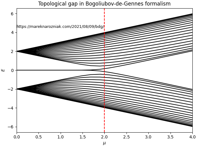
This matches the plot from Topology in Condensed Matter course nicely! We can observe the topological gap opening at .
The energy spectrum obtained from Hamiltonian is exact in the sense that in our case it provides energies of a single fermion in the 1D chain. From those energies of the multi-fermion system can be obtained by computing all binomial combinations of those energies. It is exact in the sense that it provides all the necessary information to recreate the full energy spectrum of the multi-fermion system.
The full source code of this simulation is published under an MIT license on GitHub. If you find errors please tweet me and let me know.