Topological Teleportation
Share on:Quantum teleportation (Bennett et al., 1993) has already been covered on this blog. This was the first tutorial I have written on this website. Right now we are going to re-visit this concept again from a slightly different perspective. Recently we have been talking a lot about the Majorana zero modes, creating them using the topological phase transitions and performing quantum computation by braiding them defining the Majorana qubits. The question to ask now is, would it be possible to perform the quantum teleportation on such states defined on the Kitaev chains? In other words, could we teleport a state from one Kitaev chain onto another using nothing else but braids of their edges? Turns out yes!
It was June 5th, 2019. Very fun time as Jonathan Dowling visited us in Shanghai to be a speaker at ITU Workshop on Quantum Information Technology (QIT) for Networks. At our lab, we all joined and attended it. During the break time, I was chatting with my Ph.D. advisor Tim Byrnes, we discussed teleporting states in the Kitaev chains and we got quite excited about this idea. It took us quite a few months to develop a necessary theory to make it work, which eventually resulted in the PRL publication (Huang et al., 2021) which additionally has been highlighted on the NYU Shanghai website.
The key to performing quantum teleportation is the ability to perform entangling operations. As we have few entangling gates described in (Narozniak, Dartiailh, Dowling, Shabani, & Byrnes, 2021) and also in this tutorial we found that the inner braid equivalent to operation does produce the effect of quantum teleportation with slightly different classical correction.
We start by producing the entangled state. Working in the logical space we begin by creating entanglement between second and third logical qubits using inner braid which corresponds to operation
The first logical qubit contains the state to be teleported , which can be written as
Now after applying the gate we have
from which we can deduce what corrections have to be applied depending on the measurements of the first two logical qubits. Under the form of a logical circuit, those and corrections depending on measurements are

The rightmost logical qubit is prepared in the logical state to avoid getting entangled with the rest of the system in case the -correction getting applied. The teleportation itself is performed entirely using the braiding operations, however classical correction requires the logical -operation needs an extra qubit.
I did this tutorial slightly differently than we described in the paper. Here we do not simply assume the existence of such an ancilla Kitaev chain, we also prepare it. If we include the state preparation an extra ancilla topological qubit is required and one more inner braid

The above diagram contains classical correction operators which of course do not need to always be applied. To more formally define the measurement we will prepare appropriate projection operators. But first, a topological qubit on logical -basis could be written as
where . For the final state after the teleportation if the first topological qubit has been measured to be and second we could define the projection operator
which gives us the post-teleportation and post-measurement state
we could trace out logical qubits apart from the teleported logical qubit on the third side and get fidelity for each of the outcomes as
This was for the case of topological qubits each of length . The partial trace arguments would need to be adjusted for different system sizes. I have numerically simulated the above approach and feel free to review the Python source code. The bar plot comparing fidelities for the cases with and without classical correction are as follows
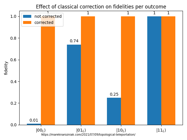
The exact distribution depends on the random state. There would always be one outcome with perfect fidelity as there is one outcome that does not require any classical correction.
Today we have simulated the topological teleportation by applying sequences of unitary braids to topological states. The full source code of this simulation is published under an MIT license on GitHub. If you find errors please tweet me and let me know.
- Bennett, C. H., Brassard, G., Crépeau, C., Jozsa, R., Peres, A., & Wootters, W. K. (1993). Teleporting an unknown quantum state via dual classical and Einstein-Podolsky-Rosen channels. Phys. Rev. Lett., 70(13), 1895–1899. 10.1103/PhysRevLett.70.1895
- Huang, H.-L., Narozniak, M., Liang, F., Zhao, Y., Castellano, A. D., Gong, M., Wu, Y., et al. (2021). Emulating Quantum Teleportation of a Majorana Zero Mode Qubit. Phys. Rev. Lett., 126(9), 090502. 10.1103/PhysRevLett.126.090502
- Narozniak, M., Dartiailh, M. C., Dowling, J. P., Shabani, J., & Byrnes, T. (2021). Quantum gates for Majoranas zero modes in topological superconductors in one-dimensional geometry. Phys. Rev. B, 103(20), 205429. 10.1103/PhysRevB.103.205429