Topological phase transitions by braiding
Share on:The topological quantum computation has been a Holy Grail of quantum computing. A magical solution to (many) of our noisy problems and yet, to the moment of writing this tutorial it has not yet been found. Previously we briefly discussed what are those topological quantum states and why people are interested in them. We also mentioned a few words about crabs and sweet times of playing Heroes of Might and Magic III and Pokémon Silver.
If you have read the previous tutorial you have a brief idea that those topological states are represented by pairings of modes. If the state is a configuration of pairings then processing such state should consist of altering the pairings. This is what people refer to as braiding (although it does have a more strict, group-theoretical definition). In 1D, you could braid edges of pairs and using the braiding operator.
If you know QuTip and have the Majorana operators from the previous tutorial implementing this operator becomes easy
def Uij(L, g1, i, g2, j, start=0, Opers=None):
    ga = g1(L, i, start=start, Opers=Opers)
    gb = g2(L, j, start=start, Opers=Opers)
    return ((np.pi/4.)*ga*gb).expm()
Previously we have achieved a topological phase transition by performing adiabatic changes of parameters of the Kitaev Hamiltonian operator describing a one-dimensional topological semiconductor. There also exists a unitary description of such topological phase transition, after all, it is a sequence of braids that makes one of the fermions delocalized on the far edges of the 1DTS.
What we were doing last time consisted of modifying the values of onsite energy and enabling couplings between the sites. The uncoupled sites with onsite energy are regular fermions described with regular fermion operators and . If we consider a sequence of same-species local braids
we would find that applying it to the regular fermions turns them into quasifermions
which implies that same-species braids applied locally are equivalent to the adiabatic manipulations of and parameters turning into regimes. A more detailed explanation of that can be found in the Section II.E of our paper (Narozniak, Dartiailh, Dowling, Shabani, & Byrnes, 2021).
From that, we know that such phase transition is a sequence of braids acting on neighboring sites exchanging local Majorana edge modes indicated by the same species. This moves to pair further and further. For the system of length if we start with a filled state
and apply the following sequence of local braids
we obtain the highly delocalized pairing on the edges just as last time! We could simulate this effect in Python with QuTip as follows
vacuum = tensor([basis(2, 0) for j in range(L)])

filled = vacuum
for n in range(L):
    filled = ad(L, n, Opers=Opers)*filled

psi0L = filled
for i, n in enumerate(reversed(range(L-1))):
    U = Uij(L, gl, n, gl, n+1, Opers=Opers)
    psi = U*psi0L
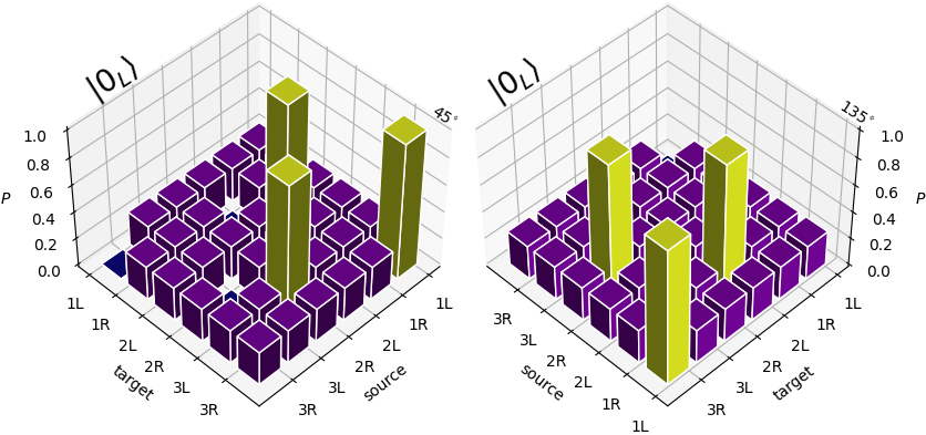
Just looking at the operators does not provide us with much intuition, however, such a topological phase transition implemented using a sequence of local braids becomes more clear once we draw a braiding diagram

and see the final state indeed possesses the Majorana Zero Modes on its edges. Numerically the results also match our previous tutorial.
They might look too perfect, but if you execute the adiabatic code yourself and shorten the adiabatic sweep time you will witness noisiness in the plots which are not there in case of a sequence of unitary braids.
The interesting thing here is that we do not need fermions to perform braids. In the Majorana picture, the difference between presence and absence is a simply different ordering of modes, which means that we could braid fermions with a lack of fermions or simply with the vacuum. Let us try it now by starting with an almost filled state, leaving one empty lattice site at the end.
We apply an exactly same unitary sequence of braids on this almost filled state
and we receive another topological regime state of the same energy. This is allowed because the ground state of the topological regime Hamiltonian is degenerate (remember why we call them zero modes?). We also verify it with Python.
psi1L = a_(L, L-1, Opers=Opers)*filled
for i, n in enumerate(reversed(range(L-1))):
    U = Uij(L, gl, n, gl, n+1, Opers=Opers)
    psi1L = U*psi1L
Visually braiding the edge of the vacuum looks the same. At the final state, the highly delocalized fermion is a lack of fermion.

Numerically exactly opposite pairing order becomes detectable.

In this sense the delocalized fermion could be labeled as logical zero state and delocalized vacuum would then be the logical one state . An arbitrary topological logical state would be then
and next time we might define some topological qubits based on those states and also some quantum gates to process them.
Today we have simulated the topological phase transitions by applying sequences of unitary braids to topological states. The full source code of this simulation is published under MIT license on GitHub. If you find errors please tweet me and let me know.
- Narozniak, M., Dartiailh, M. C., Dowling, J. P., Shabani, J., & Byrnes, T. (2021). Quantum gates for Majoranas zero modes in topological superconductors in one-dimensional geometry. Phys. Rev. B, 103(20), 205429. 10.1103/PhysRevB.103.205429