Majorana Qubits
Share on:Until now we have briefly covered some concepts of quantum computation, and condensed matter physics and we have quite an intro on the topological quantum computation. We have simulated Majorana Zero Modes inside of a 1D topology by numerically implementing the Kitaev model. We have identified different configurations of the pairing of Majorana fermions forming different topological states. We have achieved that by adiabatically varying the coefficient of the Kitaev chain model and later we achieved it again by implementing the braiding operator in topological phase transitions by braiding tutorial. However, until now none of that has performed any kind of quantum computation and that is going to be the goal of this tutorial.
The braiding operator as introduced in the latter article does not change the configuration of modes and its effect is global phase only. This indicates that designing a quantum gate would require at least two pairs of modes. Assuming two such 1D topologies with MZMs on their edges are available, we could create possible pairings, and each of those braids corresponds to a quantum gate with particular effect on the logical space. That is visually described below.

In the Figure above each square is a simplification of an entire multi-site 1D topological superconductor and gates are implemented by braiding particular edges. I will not detail why those particular pairings give those particular gates but I encourage you to read about it in our paper (Narozniak, Dartiailh, Dowling, Shabani, & Byrnes, 2021) section II.F. The detailed, but exhaustive proof of each of the eigenstates via the Jordan-Wigner transformation is provided in another of our publications (Huang et al., 2021) supplementary material section II.C.
As usual, we can proceed with a little numerical simulation. We are going to simulate the inner braid where a single 1D topological superconductor is of length and this braid is between the inner edges between the domains. As the figure above suggests that would implement the gate acting on the logical space represented by entire domains as qubits. In parallel, we would simulate the simple Hamiltonian on a two-qubit system just to compare the expectation values and demonstrate those operations are indeed equivalent.
Let us start by producing the logical state of a single 1DTS, we do it in a way the same as making psi0L and psi1L in the topological phase transitions by braiding tutorial. Given the total system, size is Ltot=2*L we define the inner inter-wire braid Hamiltonian operator
H = 0.25*1j*gr(Ltot, L-1, Opers=Opers)*gl(Ltot, L, Opers=Opers)
with particular Jordan-Wigner convention indicated in the Opers data structure. If that is not clear check previous tutorials where I have put more emphasis on explaining that concept.
The above Hamiltonian can simulate the inter-wire braid on the inner edges of Majorana zero modes, but observing any effects of that operation requires observable operators. For the initial state below being logical state
psi01L = tensor(psi0L, psi1L)
we construct logical- operator using psi0L and psi1L states as follows
lSz = psi0L*psi0L.dag() - psi1L*psi1L.dag()
lSz1 = tensor([lSz] + [qeye(2) for i in range(L)])
lSz2 = tensor([qeye(2) for i in range(L)] + [lSz])
The lSz1 and lSz2 are artificial abstract operators measuring the entire nanowires in their logical $z$-basis. Let us call them and . We also quickly jot down the qubit equivalent of the above
# qubits initial state
psi01 = tensor(basis(2, 0), basis(2, 1))

# qubit Hamiltonian
H = 0.25*Sx(2, 0)*Sx(2, 1)
For the qubits we measure operators and . We perform both time-evolutions and mark a time step
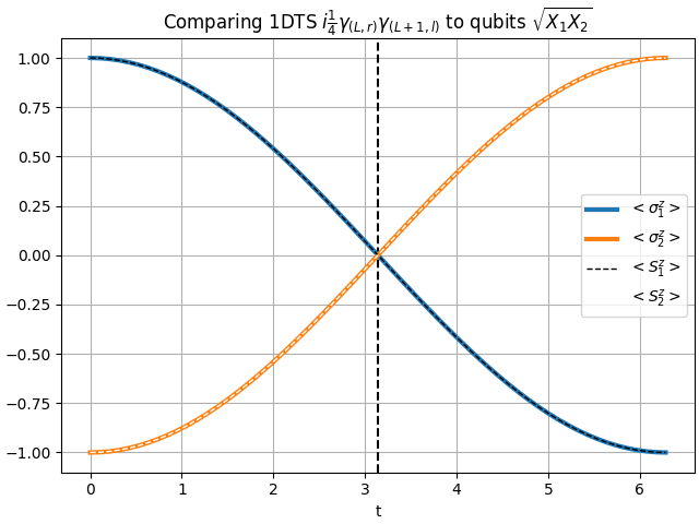
at the moment we see that gate has been applied and moreover, the 1DTS measurement match the qubit system measurement showing that is (in terms of the logical space) equivalent to . Of course the exact forms of those operators, which is not even that relevant, depends on the choice of Jordan-Wigner transformation operators.
The gates mentioned in this article are not a universal set of gates. The non-Clifford gates are not present in that set. The time-evolution we performed is an artificial, numerical simulation of something which is not achievable (or at least not easily achievable) in real life as those braids can not be fractionally applied which limits us to the operators of the form. This is not the worst as it still allows to perform some forms of quantum computation and is fully topologically protected. We will talk more about those ideas in future tutorials.
The full source code of this simulation is published under an MIT license on GitHub. If you find errors please tweet me and let me know.
- Narozniak, M., Dartiailh, M. C., Dowling, J. P., Shabani, J., & Byrnes, T. (2021). Quantum gates for Majoranas zero modes in topological superconductors in one-dimensional geometry. Phys. Rev. B, 103(20), 205429. 10.1103/PhysRevB.103.205429
- Huang, H.-L., Narozniak, M., Liang, F., Zhao, Y., Castellano, A. D., Gong, M., Wu, Y., et al. (2021). Emulating Quantum Teleportation of a Majorana Zero Mode Qubit. Phys. Rev. Lett., 126(9), 090502. 10.1103/PhysRevLett.126.090502