Majorana Zero Modes

Quantum computers could be build out of many possible candidate physical systems in a similar way as classical computers. Anything that could implement a logic gate is a candidate building block of a computer. There has even been a proposal for classical gates build out of swarms of soldier crabs (Gunji, Nishiyama, Adamatzky, & and, 2011) which is not surprising to me as crab represents a superior form in nature and as sooner or later everything would take a form of a crab due to the process of carcinisation. That includes computers. I am not entirely clear on what quantum field of crabs would be like. At the current level of knowledge in quantum physics and the zoology specialized in crustaceans those kind of questions cannot yet be answered. At the moment quantum crabs are out of reach for designing quantum logic gates, that is one of the reasons scientists have considered different options and one of the possibilities are the Majorana fermions.

Proposed in (Majorana, 1937) by and named after the Italian physicist Ettore Majorana who has disappeared in mysterious circumstances are fermions denoted here $\gamma_k$ are their own antiparticles

$\begin{aligned} \gamma_k^2 &= 1 \end{aligned}$

being purely real suggests we could use two of them to describe a single regular fermion

$\begin{aligned} a_n &= \frac{1}{2}(\gamma_{(n,l)} + i \gamma_{(n,r)}) \\ a_n^\dagger &= \frac{1}{2}(\gamma_{(n,l)} - i \gamma_{(n,r)}) \end{aligned}$

Thus a single fermionic site could contain two of such Majorana fermions which is denoted by what we like to call species and on site $n$ it could be left $\gamma_{(n,l)}$ or right $\gamma_{(n,r)}$. The Majorana fermions are fermions thus

$\begin{aligned} \{\gamma_{(n,\sigma)}, \gamma_{(n^\prime,\sigma^\prime)}\} &= 2 \delta_{n,n^\prime} \delta_{\sigma,\sigma^\prime} \end{aligned}$

it is also possible to do the other way around, define the Majorana fermions in terms of the regular fermions

$\begin{aligned} \gamma_{(n,l)} &= a_n + a_n^\dagger \\ \gamma_{(n,r)} &= -i a_n + i a_n^\dagger \end{aligned}$

or even design new sorts of fermions by pairing Majoranas differently than in the nearest neighbour fashion, let us call those weirded fermions the quasifermions

$\begin{aligned} f_{\alpha,\beta} &= \frac{1}{2}(\gamma_\alpha + i \gamma_\beta) \\ f_{\alpha,\beta}^\dagger &= \frac{1}{2}(\gamma_\alpha - i \gamma_\beta) \end{aligned}$

obeying the

$\begin{aligned} f_{\alpha,\beta} &= -i f_{\beta,\alpha} \end{aligned}$

Back in 2001, I was spending most of my time playing Heroes of Might and Magic III and Pokémon Silver and I didn’t even have a clue that Alexei Kitaev (Kitaev, 2001) had proposed a one-dimensional system in which a pairing of Majorana fermions occurs on the far edges and has zero energy. How would I… I was 11 and for me it was still pre-internet era. The Hamiltonian proposed by Kitaev takes form

$\begin{aligned} H = -\frac{1}{2} \mu \sum_j^L (2 a_j^\dagger a_j - 1) - \sum_j^{L-1} [w (a_j^\dagger a_{j+1} + a_{j+1}^\dagger a_j) - \Delta a_j a_{j+1} - \Delta^\ast a_{j+1}^\dagger a_j^\dagger)] \end{aligned}$

and under specific conditions (modeled by a choice of parameters $\mu$, $w$ and $\Delta$) it enters a regime with a quasifermion delocalized between the far edges of the one-dimensional geometry. The $\mu$ terms is the onsite energy or chemical potential on the modelized nanowire. Then $w$ would be the electron hopping and finally $\Delta$ the induced superconducting gap. According to this theory, sufficiently small $\mu$ compared to $w$ and $\Delta$ would make this system transit from the trivial regime into the topological regime. The form of the Hamiltonian stated above tells me nothing about the pairings on the chain which is why I prefer to work with the Majorana fermion form.

$\begin{aligned} H = -\mu \sum_j^L & i \gamma_{(j,l)} \gamma_{(j,r)} \\ - \frac{1}{2} \sum_j^{L-1} &[w (i \gamma_{(j,l)} \gamma_{(j+1,r)} - i \gamma_{(j,r)} \gamma_{(j+1,l)}) \\ - & (\Delta - \Delta^\ast) \gamma_{(j, l)} \gamma_{(j+1,l)} - i (\Delta + \Delta^\ast) \gamma_{(j, l)} \gamma_{(j+1,r)} - i (\Delta + \Delta^\ast) \gamma_{(j, r)} \gamma_{(j+1,l)} - (\Delta - \Delta^\ast) \gamma_{(j, r)} \gamma_{(j+1,r)}] \end{aligned}$

this is much better but still there are too many possible pairings simultaneously thus for purely aesthetic reasons we may take the assumption $\Delta \in \mathbb{R}$ and $\Delta = -w$ and the Hamiltonian simplifies into the form

$\begin{aligned} H \Bigr|_{\Delta = -w} = -\mu \sum_j^L & i \gamma_{(j,l)} \gamma_{(j,r)} - w \sum_j^{L-1} \gamma_{(j, r)} \gamma_{(j+1,l)} \end{aligned}$

which is simple once you know how to associate those terms with the pairings in the one-dimensional geometry according to the convention visually illustrated as follows

Let us establish that left-to-right pairing is a fermion while right-to-left pairing is a hole or a lack of fermion. According to the theory if $\mu < 2 w$ the inter-site couplings would dominate the on-site couplings and system would enter the topological phase. Regardless if it is trivial or topological phase, the number of fermions has to be conserved but the Hamiltonian in the Majorana fermionic form describes $L-1$ fermions thus one of them is the zero energy quasifermion and if you examin the couplings you will conclude that it is the outer edges pairing one.

In this tutorial we are going to numerically simulate that topological phasa transition and numerically estimate the probability of detection of different pairings within the one-dimensional geometry. As a basis for the code we would re-use a lot of methods from Jordan-Wigner transformation tutorial.

We can produce initial state being a trivial regime of $L=3$ regular fermions

$\begin{aligned} \left \vert \psi_0 \right> = \prod_{j=1}^{L} a^\dagger_j \left \vert 0 \right>_N \end{aligned}$

why with $\left \vert 0 \right>_N$ we indicate what we refer to as the trivial vacuum or just vacuum. The meaning of the subscript will become more significant in the future tutorials and at this stage it is fine to simply ignore it.

What we are going to do is create topological regime with a highly delocalized quasifermion $f_{(1,l),(L,r)}$ on the edges of the one-dimensional topological semiconductor of length $L=3$.

$\begin{aligned} H^{(N)}_j &= 2 a_j^\dagger a_j - 1 \\ H^{(T)}_j &\Bigr|_{\Delta = -w} = a_j^\dagger a_{j+1} + a_{j+1}^\dagger a_j - a_j a_{j+1} - a_{j+1}^\dagger a_j^\dagger \end{aligned}$

we wish to achieve the following pairings

to do so we will decrease $\mu$ site by site starting from rightmost site to the left. First step would be to decrease the rightmost $\mu$ and then consecutively decrease following once while increasing $w$. While couplings are off initially, there is no interaction between the sites. That is because we want to achieve high fidelity and we do not care about experimental realisability (I do not want reality, I want magic!). Think of those sites as completely isolated and gradually connected into something which happens to have a topology of a 1D chain. For each adiabatic step the Hamiltonians are

$\begin{aligned} H_0 &= H^{(N)}_1 + H^{(N)}_2 + H^{(N)}_3 \\ H_1 &= H^{(N)}_1 + H^{(N)}_2 \\ H_2 &= H^{(N)}_1 + H^{(T)}_2 \\ H_3 &= H^{(T)}_1 + H^{(T)}_2 \end{aligned}$

visually

and for each of them

$\begin{aligned} H(\lambda) &= ((1-\lambda) H_i + \lambda H_f) \Bigr|_{-\Delta = w = \mu = 1} \end{aligned}$

If that confuses you I recommend to check my tutorial on quantum adiabatic optimization which provides an introduction to how to numerically simulate those quantum adiabatic transitions with QuTip. In Python we would first define the length of the chain, make the choice for the Jordan-Wigner operators and prepare lambda functions of the operators for a more convenient notation

# length of the 1D topological semiconductor
L = 3

# Jordan-Wigner choice to have |0> as the vacuum
Opers = Sz, Sy, Sx

# prepare operators for more readable notation
a_ = lambda n: op_a_(L, n, Opers=Opers)
ad = lambda n: op_ad(L, n, Opers=Opers)

Now produce vacuum state for Jordan-Wigner choice made and define filled state as well.

# produce a vacuum state
vac = basis(2, 0)
vacuum = tensor([vac for j in range(L)])

# produce a completely filled state
filled = vacuum
for n in range(L):
    filled = ad(n)*filled

Define Hamiltonians for each of the adiabatic steps, they rely on the topological regime terms as well which if defined as lambda functions simplify the notation even further.

# Topological terms in the Hamiltonian
Hhop = lambda n: ad(n+1)*a_(n)+ad(n)*a_(n+1)
Hbcs = lambda n: a_(n)*a_(n+1)+ad(n+1)*ad(n)

# Hamiltonian steps
H0 = -0.5*(2*ad(0)*a_(0)+2*ad(1)*a_(1)+2*ad(2)*a_(2)-3)
H1 = -0.5*(2*ad(0)*a_(0)+2*ad(1)*a_(1)-1)
H2 = -0.5*(2*ad(0)*a_(0)-1)+Hhop(1)-Hbcs(1)
H3 = Hhop(0)-Hbcs(0)+Hhop(1)-Hbcs(1)

We can define simulation parameters and perform the adiabatic sweeps for each of the transitions.

# prepare the simulation
tau = 10.*np.pi
resolution = 300
times = np.linspace(0., tau, resolution)
opts = Options(store_final_state=True)

# perform the transitions
psi0 = filled

Ht = lambda t, args: (1-t/tau)*H0 + (t/tau)*H1
psi1 = mesolve(Ht, psi0, times, options=opts).final_state

Ht = lambda t, args: (1-t/tau)*H1 + (t/tau)*H2
psi2 = mesolve(Ht, psi1, times, options=opts).final_state

Ht = lambda t, args: (1-t/tau)*H2 + (t/tau)*H3
psi3 = mesolve(Ht, psi2, times, options=opts).final_state

As for the measurements we can define the number operator that checks particular pairing of Majorana fermions

$\begin{aligned} N_{\alpha,\beta} &= f^\dagger_{\beta,\alpha} f_{\beta,\alpha} \end{aligned}$

and we can calculate expectation value of this operator for each of the possible pair in the $L=3$ chain for the states $\left \vert \psi_1 \right>$, $\left \vert \psi_2 \right>$ and $\left \vert \psi_3 \right>$ and we get

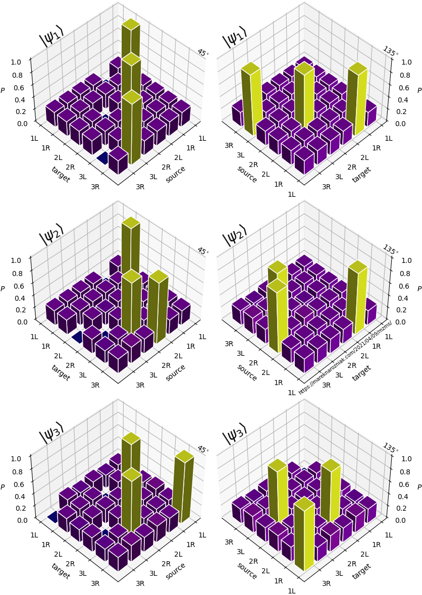
which reproduces the pairings we wanted to achieve! We can see that $\left \vert \psi_1 \right>$ pairs each of the onsite Majorana fermions from left to right which indicates a trivial regime of the completely filled state. In the $\left \vert \psi_3 \right>$ we see the pairing between outer edges of the chain is detectable indicating the system entered the topological regime predicted by Kitaev.

To conclude, we have implemented the Kitaev chain Hamiltonian and numerically simulated the phase transition between its trivial phase and topological phase. Using the expectation values of Majorana-based number operators $N_{\alpha,\beta}$ we have shown that highly delocalized excitations occur at the boundaries of the one-dimensional geometry. In the future we can cover subjects related to quantum computation using those zero-energy modes by performing various braids. Similarly as done in our own work (Huang et al., 2021). We did not go too deep in the theory as our goal was to focus on numerics. If you are interested in knowing more about it I recommend to check the materials for the topology in condensed matter class and please compare how much time you have to wait for their $\LaTeX$ to load compared to my website.

The full source code of this simulation is published under MIT licence on GitHub and fermionic properties are tested by Travis. Also, as usual I take no responsibility for my algebra… If you find errors please tweet me and let me know. I take no responsibility for failed homework which are copy-paste from my website!

1. Gunji, Y.-P., Nishiyama, Y., Adamatzky, A., & and. (2011). Robust Soldier Crab Ball Gate. Complex Systems, 20(2), 93–104. 10.25088/complexsystems.20.2.93
2. Majorana, E. (1937). Teoria simmetrica dell’elettrone e del positrone. Il Nuovo Cimento, 14(4), 171–184. 10.1007/bf02961314
3. Kitaev, A. Y. (2001). Unpaired Majorana fermions in quantum wires. Physics-Uspekhi, 44(10S), 131–136. 10.1070/1063-7869/44/10s/s29
4. Huang, H.-L., Narozniak, M., Liang, F., Zhao, Y., Castellano, A. D., Gong, M., Wu, Y., et al. (2021). Emulating Quantum Teleportation of a Majorana Zero Mode Qubit. Phys. Rev. Lett., 126(9), 090502. 10.1103/PhysRevLett.126.090502

[Back to Top]