Quantum Adiabatic Optimization

Today we are going to learn how to simulate the process of quantum adiabatic computation and how it could be used in practice. I don’t want to make another quantum adiabatic simulation that is just like all other simulations I encountered… Random meaningless problem instance, simulate sweep, plot spectral gap… I want to solve something cool… Lets pick up the Pokémon maps problem we solved earlier in Vertex Covers and Independent Sets in game level design article only this time instead of brute-forcing by recursive enumeration lets use Adiabatic Quantum Computing (AQC) approach to solve it and find the matching solutions. First, some brief introduction to the subject.

In optimization, we usually do not think much about hardware, we focus more on abstract mathematics, heuristics, and algorithms to explore the decision space to find better candidate solutions. By contrast, Adiabatic Quantum Computing (AQC) is an optimization technique which naturally is more hardware oriented. Introduced by (Farhi, Goldstone, Gutmann, & Sipser, 2000) has been shown capable of solving NP-Hard problems (Farhi et al., 2001).

The reason why I claim this technique is more hardware oriented is because, at least to my understanding, the process of solving is a physical process - taking advantage of the adiabatic theorem (Born & Fock, 1928).

In simple terms, imagine encoding an arbitrary solution of the problem using some configuration of a physical system. To distinguish quality of those configurations we need to enforce some criterion of quality, usually minimization or maximization of objective function, for AQC this criterion is energy of the system’s configuration - the global minimum solution for objective function would become a minimum energy configuration of this physical system - known as its ground state.

In order to encode our problem in terms of AQC, we would need to design a physical system for which energy configuration corresponds to value of objective function, that would be a quantum adiabatic processor or quantum annealer. How such device would find this global minimum or ground state?

This is where the adiabatic theorem comes in handy - in simple terms it states that a physical system subject to changes, will adapt its configuration to those changes as long as they occur sufficiently slowly. Practically, we could initiate our processor in the ground state of some trivial problem - one which is easy to find - and slowly vary the parameters transforming the conditions to ones corresponding to the difficult problem one we intend to solve, and according to the adiabatic theorem, as long as those changes occur slowly, system’s configuration will adapt to those changes ending up in the ground state of the hard problem!

Of course there are some limitations, this works as long as there exists an energy gap in the transition spectrum and efficiency depends on the size of this spectral gap.

The initial configuration of the system is described by the initial problem Hamiltonian. We have freedom to choose initial problem Hamiltonian to any Hamiltonian we are capable of predicting and producing the ground state. For this tutorial I am going to use the following.

$H_I = \sum_i \sigma^x_i$

The ground state of this Hamiltonian is $\left \vert \psi_0 \right> = \left \vert -- \dots - \right>$, which could be deduced from the form of the $H_I$. That was the physical system corresponding to the initial (trivial) problem, now the Hamiltonian for the final (hard) problem.

$H_F = -\sum_{ij} J_{ij} \sigma^z_i \sigma^z_j -\sum_{i} k_i \sigma^z_i$

It is straightforward to construct $H_F$ for any optimization problem by choosing appropriate $J_{ij}$ coefficients, however finding its ground state energy is challenging. The ground state of $H_F$ is encodes the solution to the problem and can be found using the adiabatic theorem by slowly transforming $H_I$ into $H_F$.

$H(\lambda) = (1-\lambda) H_I + \lambda H_F$

By varying parameter $\lambda$ over time we transform one system into into another and if we do it slowly enough, according to adiabatic theorem, physical system (state) will have enough time to adapt and will end up in the ground state of the final Hamiltonian $H_F$ which encodes the unknown solution to our problem!

The slowless or adiabacity of this transformation can be defined as the total transition time, let us denote it as $\tau$ and in Python we will represent it as T parameter variable.

Previously we played a little bit with game map design problem related to the minimum vertex cover and maximum independent set problem, have a look at this article - Vertex Covers and Independent Sets in game level design if you haven’t yet checked it as we will extensively use the definitions from it.

From this article we learned how to define minimum vertex cover and maximum independent set problems and how they can be used for modelling, we also got a cool problem that we can solve now and compare our solutions - the Pokémon Center placing problem!

In order to solve those problems using a quantum adiabatic processor we need to find a Hamiltonian $H_F$ that encodes the solution in its ground state.

The final Hamiltonian $H_F$ as we defined it is encoded entirely in the $Z$-basis, which is (almost) convenient to define the decision space as boolean variables. Almost - because the $\sigma^z$ operator collapses the state $\left\vert\psi \right>$ into values $\{-1, 1\}$, working with this domain is… Weird? At least to me, it feels counter intuitive to work with such values of variables and it makes much more sense to work with $\{0, 1\}$ domain, fortunately we can introduce a little hack to shift the energy from the spin-$\frac{1}{2}$ domain into good old boolean domain! Let us introduce a boolean domain operator.

$B_i = \frac{1}{2}(1-\sigma^z_i)$

This operator is a lot more convenient in defining models for problems as it collapses into $\left<\psi \vert B \vert \psi \right> \in \{0, 1\}$ domain. Using this operator we can define our first Hamiltonian solving the minimum vertex cover, recalling the definition, minimum vertex cover is violated of there is an edge of the graph such that both vertices it connects are not selected and we intend to select as little as possible. Using our boolean quantum variables we come up with the following.

$H_F^\text{MVC} = J\sum_{ij \in E(G)} (1-B_i)(1-B_j) + k \sum_{i \in V(G)} B_i$

It is based on a fact that $(1-B_i) = 1$ if $B_i=0$, it reverses the effect of $B_i$. This is raising the systems energy by a single unit $J$ if there is an edge that has both vertices non selected, moreover, every selected vertex is raising the energy by unit of $k$ so the ground state energy will try to have as few of them selected as possible. It is important to have $k < J$ because otherwise it would become profitable to violate constraints by selecting fewer vertices and it would trivialise the solver. If you wonder why is that try to draw the simplest graph of single edge and two vertices and calculate the energy for different cases.

Now let us try the maximum independent set in this boolean domain. From the previous article - Vertex Covers and Independent Sets in game level design - we know how those problems relate and how one can be converted into another, which translate really nicely to how transform those models. As this time it is a maximization problem, selecting more vertices should decrease the energy and constraint will be violated if both are selected - just following the definition of the maximum independent set!

$H_F^\text{MIS} = J\sum_{ij \in E(G)} B_i B_j - k \sum_{i \in V(G)} B_i$

The boolean domain made it a lot easier to create those models, yet if we expand those Hamiltonians into spin form we will notice constant terms which do not really contribute to the problem and we can get rid of them without losing any features. The above Hamiltonians in spin form without the constant terms look as follows.

$\begin{aligned} H_F^{\prime\text{MVC}} &= J\sum_{ij \in E(G)} (\sigma^z_i + \sigma^z_j + \sigma^z_i \sigma^z_j) - k \sum_{i \in V(G)} \sigma^z_i \\ H_F^{\prime\text{MIS}} &= J\sum_{ij \in E(G)} (-\sigma^z_i - \sigma^z_j + \sigma^z_i \sigma^z_j) + k \sum_{i \in V(G)} \sigma^z_i \end{aligned}$

This is a good moment to start coding, defining those Hamiltonians and checking the energy spectra to see if they solve our Pokémon Center placing problem! Let us start with the required imports and operators.

# Identity operator
def Is(i): return [qeye(2) for j in range(0, i)]

# Pauli-X acting on ith degree of freedom
def Sx(N, i): return tensor(Is(i) + [sigmax()] + Is(N - i - 1))

# Pauli-Z acting on ith degree of freedom
def Sz(N, i): return tensor(Is(i) + [sigmaz()] + Is(N - i - 1))

# a quantum binary degree of freedom
def x(N, i):
    return 0.5*(1.-Sz(N, i))

There is a trick you can do to be able to write nice Hamiltonians in Python using notation similar to one we use on paper. We need a sum operator that works with generic object type, this will allow to just put QuTip operators there and let it calculate the sum of them!

def osum(lst): return np.sum(np.array(lst, dtype=object))

Now using those we can define the Hamiltonians. Each of them will be a Python function returning the operator, it will accept the system size and graph edge pairing indices.

# minimum vertex cover Hamiltonian,
def HMVC(N, pairs):
    Hq = osum([(1. - x(N, i))*(1. - x(N, j)) + (1. - x(N, j))*(1. - x(N, i)) for i, j in pairs])
    Hl = 0.99*osum([x(N, i) for i in range(N)])
    return Hq + Hl

# minimum vertex cover Hamiltonian, no constant shift version
def HMVC_(N, pairs):
    Hq = osum([Sz(N, i) + Sz(N, j) + Sz(N, j)*Sz(N, i) for i, j in pairs])
    Hl = - 0.5*osum([Sz(N, i) for i in range(N)])
    return Hq + Hl

# maximum independent set Hamiltonian,
def HMIS(N, pairs):
    Hq = osum([x(N, i)*x(N, j) + x(N, j)*x(N, i) for i, j in pairs])
    Hl = - 0.99*osum([x(N, i) for i in range(N)])
    return Hq + Hl

# maximum independent set Hamiltonian, no constant shift version
def HMIS_(N, pairs):
    Hq = 2.*osum([-Sz(N, i) - Sz(N, j) + Sz(N, i)*Sz(N, j) for i, j in pairs])
    Hl = 0.5*osum([Sz(N, i) for i in range(N)])
    return Hq + Hl

We can extract data from our set instance like this, mind the fact that Kanto region instance is defined using frozen sets, thus when you convert it to lists there is no guarantee order will be preserved. The way I deal with this problem is I convert the instance into lists and pickle them into a file and then I load them from this file so that same indices get preserved for all the runs.

Problem Hamiltonians are purely diagonal, but still lets use proper methods for diagonalizing them. We will do it in a similar way as when we plotted the dispersion relation of the 1D Tight Binding Model, even if meaning is not even close to what we are doing now, procedure is practically the same as we just need to find the energy spectrum. The first five lowest energies of spectrum of each of the Hamiltonians we considered earlier are listed here below.

$H_F^\text{MVC}$	Energy	Size MIS	Size VC	$H_F^{\prime\text{MVC}}$	Energy	Size MIS	Size VC	$H_F^\text{MIS}$	Energy	Size MIS	Size VC	$H_F^{\prime\text{MIS}}$	Energy	Size MIS	Size VC
0	5.94	6	6	0	-15.0	6	6	0	-5.94	6	6	0	-30.0	6	6
1	5.94	6	6	1	-15.0	6	6	1	-5.94	6	6	1	-30.0	6	6
2	5.94	6	6	2	-15.0	6	6	2	-5.94	6	6	2	-30.0	6	6
3	6.93	5	7	3	-14.0	5	7	3	-4.95	5	7	3	-29.0	5	7
4	6.93	5	7	4	-14.0	5	7	4	-4.95	5	7	4	-29.0	5	7

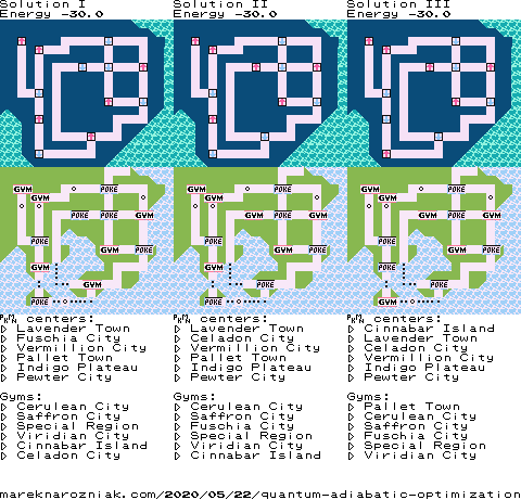
We can see that the ground state is degenerate, there are three states of the lowest energy, which is consistent with our earlier findings! Even if we haven’t seen the solution we could still deduce those are optimal as we can see how the size of minimum vertex cover increases as we go higher in energy and same with maximum independent set which decreases in size as the energy grows.

The top three lowest energy solutions from $H_F^{\prime\text{MIS}}$ Hamiltonian can be visualized and compared to our classical solution based on recursive enumeration we have found earlier and they match exactly. The top row are quantum solutions with spins up and spins down and bottom row are the matching previously obtained solutions.

Now let us proceed with the adiabatic method, we can use the $H_F^{\prime\text{MIS}}$ as our final problem Hamiltonian. Together they form a time-dependent Hamiltonian, the time-dependence can be conveniently defined using Python’s Lambda expressions. We should also define some parameters such as total sweep time, for which we can take $\tau = 25\pi$, being the number of revolutions around the Bloch sphere.

tmax = 25.
T = tmax*np.pi

Hi = -osum([Sx(N, i) for i in range(N)])
Hf = HMIS_(N, pairs)

H = [[Hi, (lambda t, args: 1. - t/T)], [Hf, (lambda t, args: t/T)]]

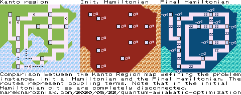
For the Pokémon instance the initial and final Hamiltonians can be visualized as follows.

Before we run the solver we have to define a callback measurement function, which will be called at each numerical step and gather measurement data which can later be plotted and used for analysis of the results. Initially, let us just gather the information about the total energy of the system, this is just an expectation value of the time-dependent Hamiltonian $E = \left<\psi_t\vert H(t) \vert\psi_t\right>$ and can be evaluated as follows.

def measureEnergy(t, psi):
    # evaluate time-dependent part
    H_t = qobj_list_evaluate(H, t, {})
    return expect(H_t, psi)

Where H is the Hamiltonian involving Lambda expressions, the qobj_list_evaluate will evaluate those expressions at given t to get a matrix form Hamiltonian which can be used to take the expectation value of. This callback is sufficient to define the measurement of the energy and we can launch the numerical simulation of the adiabatic sweep. Lets not forget about creating an initial state which is the ground state of $H_I$, just as a reminder in our case it is $\left \vert \psi_0 \right > = \left \vert --\dots -\right>$.

minus = (basis(2, 0) - basis(2, 1)).unit()
psi0 = tensor([minus for i in range(N)])

res = 300
times = np.linspace(0., T, res)
opts = Options(store_final_state=True)
result = mesolve(H, psi0, times, e_ops=measureEnergy, options=opts)

The result will contain the final state and list of all the measurements of energy. Lets plot them!

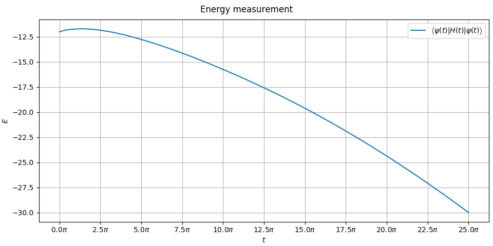
This energy plot is not as meaningful to us because we have not plotted exact ground state level and excited state level. Hamiltonian is time-dependent so we would have to do it at each numerical step (which we have 300 of, to have nice resolution of the plots) and our problem involves twelve qubits… There are plenty of quantum adiabatic tutorials on the internet that plot the spectral gap of some trivially small instances. We are not here to admire gaps, here we simulate solving a meaningful instance of Pokémon problem! We see the energy starts at $E_0 = -12$ and ends at $E_F = -30$ which is the ground state energy of $H_F^{\prime\text{MIS}}$.

So far we know the Hamiltonian has a degenerate ground state composed of three solutions which matches our brute force results from previous article and we know that the adiabatic sweep has led us to state of that energy, it means that the final state of our adiabatic sweep must be some superposition of the solution to our problem. We can cheat a little bit as we know what solutions are and extract them and calculate the probabilities of measuring each of them. Long time ago, in the first article of this blog, we simulated the quantum teleportation protocol and used fidelity as a metric if teleported state matches. This time we will use exactly the same metric to check how the final state overlaps with the expected state we found classically using brute-force earlier.

We can check the fidelity of every possible spin configuration of system of size $N=12$ using the following function.

def extractFidelities(N, ket, top):
    # produce all possible binary configurations of length N
    configurations = list(itertools.product([0, 1], repeat=N))
    fidelities = np.zeros(2**N)
    for i, configuration in enumerate(configurations):
        refket = tensor([basis(2, value) for value in configuration])
        fidelity = np.abs(refket.overlap(ket))**2.
        fidelities[i] = fidelity
    # get the indices highest fidelities
    best = (-fidelities).argsort()[:top]
    # return those configurations and corresponding fidelities
    return [configurations[c] for c in best], [fidelities[c] for c in best]

If we run it with result.final_state and top=10 we will see a list of top ten most likely outcomes that can be measured after the adiabatic sweep. We know the solutions have the energy of $E_F = -30$ so let us also display the energy of each of those top ten most likely outcomes which will allow us to identify which of those outcomes are the solutions to the Pokémon problem.

$\left \vert \psi \right >$	Fidelity	Energy
$\left \vert001100111100\right >$	0.49766	-30.0
$\left \vert001001111100\right >$	0.25033	-30.0
$\left \vert011100101100\right >$	0.2481	-30.0
$\left \vert001100101100\right >$	0.00047	-29.0
$\left \vert010100100011\right >$	0.00041	-29.0
$\left \vert000100111100\right >$	0.00037	-29.0
$\left \vert001100111000\right >$	0.00034	-29.0
$\left \vert010100101010\right >$	0.00029	-29.0
$\left \vert001001101100\right >$	0.00021	-29.0
$\left \vert110100001010\right >$	0.00018	-29.0

The top three most likely solutions also happen to be ones with energy $E_F = -30$ and they are a lot more likely than any other configuration, their accumulated measurement probability adds up to $P=0.99608$ which makes it almost certain that after running our adiabatic quantum processor by transforming $H_I$ into $H_F$ over the total time of $\tau=25\pi$ there is probability of $P=0.99608$ that we will measure one of three solutions to the Pokémon problem!

Now the fact that we measure a right solution is almost certain, yet what is interesting is that the distribution of measurement probability between those three solutions is not uniform. One of them is twice more likely then each of the other ones. I purposely do not explicitly say which one is it as the ordering of indices of the graph is arbitrary as the graph is based on set definition.

We can study how this fidelity evolves over the course of adiabatic sweep by implementing a new measurement callback function. The previous measurement callback function was only measuring the total energy of the system, now we can also measure the fidelities of the (now known!) optimal solutions. Lets assume that spin configurations of the optimal solutions are stored as lists of zeros and ones inside of a list named sol_kets.

def measureEnergyFidelities(t, psi):
    # evaluate time-dependent part
    H_t = qobj_list_evaluate(H, t, {})
    # get current energy of the system
    energy = expect(H_t, psi)
    # get fidelity of all the solutions
    fidelities = []
    for ket in sol_kets:
        fidelity = np.abs(psi.overlap(ket))**2.
        fidelities.append(fidelity)
    return tuple([energy] + fidelities + [np.sum(fidelities)])

This measurement function returns energy, each of the individual solution fidelities and a sum of fidelities. We can run the adiabatic sweep, say, $20$ times for $\tau \in [\pi, 25\pi]$, assign a color for each sweep time and plot those fidelities all together.

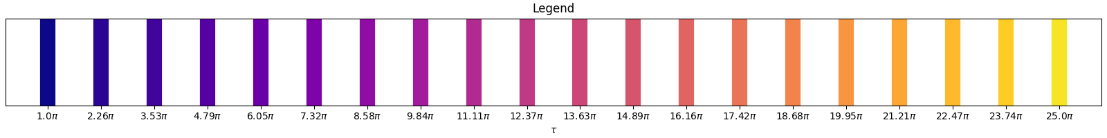
We run the adiabatic sweep again, once for each adiabatic sweep times. The fidelity plots associated to each run are available here below.

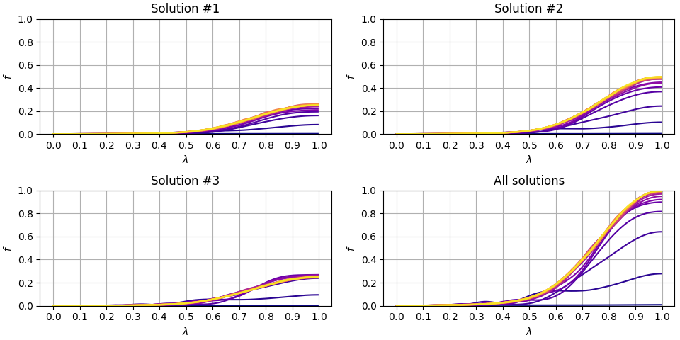
Plot is sufficiently accurate to indicate that fidelity, or probability of measuring the optimal solution, starts to approach $1$ when adiabatic sweep is of length $\tau=10\pi$ which is less than a half of the time we used earlier.

I think this is all I have to say regarding the Adiabatic Quantum Computation. To summarize, we simulated the adiabatic sweep and found a solution that matches our previous results perfectly. We learned how to create models for optimization problems, how to use the spin-$\frac{1}{2}$ and boolean domains and how to switch between them. We also learned how to examine the energy spectra of our problem Hamiltonian. Most of the code required to run those examples is not included on this page, but you can check in this this public gist repository.

As usual, if you find typos, errors, something is not clear, something is wrong, do not hesitate to let me know and feel free to tweet me!

1. Farhi, E., Goldstone, J., Gutmann, S., & Sipser, M. (2000). Quantum Computation by Adiabatic Evolution.
2. Farhi, E., Goldstone, J., Gutmann, S., Lapan, J., Lundgren, A., & Preda, D. (2001). A Quantum Adiabatic Evolution Algorithm Applied to Random Instances of an NP-Complete Problem. Science, 292(5516), 472–475. 10.1126/science.1057726
3. Born, M., & Fock, V. (1928). Beweis des Adiabatensatzes. Zeitschrift für Physik, 51(3), 165–180. 10.1007/BF01343193

[Back to Top]