The 1D Tight-Binding Model

I want to write some numerical quantum tutorials on simulating fermionic systems. I have been looking for something simple enough to get started, a while ago I did reproduce some elementary results on 1D Tight-Binding approximation and decided it would be good to turn it into a tutorial. I also hope it might be helpful to someone dealing with homework 😏.

In this tutorial we are going to find the dispersion relation of one-dimensional string of atoms subject to a Tight-Binding approximation. We will do it theoretically by taking some theoretical assumptions, then we will numerically diagonalize the Hamiltonian and demonstrate results are matching. We expect the resulting dispersion relation to reproduce a Figure 11.2 from (Simon, 2013) page 102.

Let us consider a one-dimensional model of electrons hopping between atoms, where distance between atoms is labeled as $a$, and $n$ represents a lattice site index as $\left\vert n \right>$ for $n = 1 \dots N$.

Let us assume those orbitals are orthonormal ($\left<n\vert m\right> = \delta_{n,m}$) and also let us acknowledge the presence of an onsite energy $\epsilon$ on each atomic site of this one-dimensional chain of atoms and a hopping matrix element $-t$ representing a tendency of neighboring orbitals to overlap.

It can all be summarized to

$\left<n\vert H\vert m \right> = \begin{cases} \epsilon, & \text{if}\ n=m \\ -t, & \text{else if}\ n=m \pm 1 \\ 0, & \text{otherwise} \end{cases}$

For the theoretical solution, we will apply the variational principle. If $\left\vert\psi^\prime \right>$ is a plane-waves trial wavefunction for a two-level system, it can be generalized to $\left\vert\psi \right>$, an arbitrary number of levels $N$ trial wavefunction.

$\begin{aligned} \left| \psi \right> = c_1 \left|0\right> + c_2 \left|1\right> \rightarrow & \left| \psi \right> = \sum_j^N c_j \left|j\right> \\ & \left| \psi_j \right> = c_j \left|j\right> \end{aligned}$

And from the defined earlier Hamiltonian we have

$\begin{aligned} \left<i\left|H\right|j\right> &= \epsilon \delta_{i,j} - t \delta_{i,j\pm1} \end{aligned}$

In $N=2$ case periodic boundary conditions were automatically satisfied, but for larger $N$ we need to define them

$\begin{aligned} \left<0\left|H\right|N\right> &= \left<N\left|H\right|0\right>\\ &= -t \end{aligned}$

Lets approximate the electron to be “nearly free”, thus as an intelligent guess for 1D Schrödinger equation let us fit it in a form of plane wave solution $c_n = \sqrt{N}e^{-ikx}$ where $x = na$ is quantized into multiples of $a$, and since we impose periodic boundary conditions we need the following waves to match

$\begin{aligned} \left<0\vert \psi \right> &= \left<N\vert \psi \right>\\ \sqrt{N}e^{-ika \times 0} &= \sqrt{N}e^{-ikNa} \\ 1 &= e^{-ikNa} \end{aligned}$

We can solve it for $k$, we also take into account that $N$ of possible solution differ by the integer multiple.

$k = \frac{2\pi}{Na} = \frac{2\pi}{L} \rightarrow \frac{2\pi}{a}$

We can now define $\left\vert \psi_n \right>$

$\left\vert \psi_n \right> = \sqrt{N} e^{-ik n} \left\vert n\right>$

Now we need to find the eigenenergies by solving the time-independent Schrödinger equation $H \left\vert \psi\right> = E\left\vert \psi\right>$ for $E$. Predictable form of $H$ allows us to state it as follows.

$\begin{aligned} H \left\vert \psi \right> &= \sum_n H \left\vert \psi_n \right> \\ &= \sum_n H e^{-ik na} \left\vert n \right> \\ &= \sqrt{N} \sum_n (\epsilon e^{-ik na} - t e^{-ik (n-1)a} - t e^{-ik (n+1)a}) \left\vert n \right> \\ &= \sqrt{N} \sum_n (\epsilon e^{-ik na} - t e^{ik a}e^{-ik na} - t e^{-ik a}e^{-ik na}) \left\vert n \right> \\ &= \sqrt{N} \sum_n (\epsilon - t e^{ik a} - t e^{-ik a}) e^{-ik na} \left\vert n \right> \\ &= \sqrt{N} \sum_n (\epsilon - 2t \cos(k a)) e^{-ik na} \left\vert n \right> \\ &= \sum_n (\epsilon - 2t \cos(k a)) \left\vert \psi_n \right> \end{aligned}$

We have the eigenenergies subject to assumption of orthogonality of electronic levels of nearly-free electrons. Now given that Hamiltonian we can code it in Python and see how it matches. First the dependencies.

import matplotlib.pyplot as plt
import numpy as np
from qutip import basis

Where $\sqrt{N}$ represents the normalization and eigenenergies are $E(k) = \epsilon - 2t \cos(k a)$, and it allows us to visualize the dispersion curve for electrons. Let us start by defining input parameters.

# spacing between atoms
a = 2

# number of atoms
N = 23

# total length of the 1D chain
L = N*a

# onsite energy
eps = 0.25

# hopping matrix element
t = 0.5

Now we calculate numerically the dispersion curve according to derived earlier eigenenergy expression.

k = np.linspace(-np.pi/a, np.pi/a, 2*L)
exact = eps - 2.*t*np.cos(k*a)

Let us visualize the dispersion curve using matplotlib.

xticks = np.linspace(-np.pi/a, np.pi/a, 9)
xlabels = ['' for k in xticks]
xlabels[0] = '$-\\frac{\pi}{a}$'
xlabels[-1] = '$\\frac{\pi}{a}$'

fig, axs = plt.subplots()
axs.set_xlim(-np.pi/a, np.pi/a)
axs.set_title('Tight-Binding Model, $N='+str(N)+', a='+str(a)+'$')
axs.set_ylabel('$E$')
axs.set_xlabel('$ka$')
axs.axvline(x=0., color='k')
axs.plot(k, exact, label='$E(k) = \epsilon_0 - 2 t \cos(ka)$')
axs.set_yticks([eps-2.*t, eps-t, eps, eps+t, eps+2.*t])
axs.set_yticklabels(['$\epsilon_0-2t$', '$\epsilon_0-t$', '$\epsilon_0$', '$\epsilon_0+t$', '$\epsilon_0+2t$'])
axs.set_xticks(xticks)
axs.set_xticklabels(xlabels)
axs.legend()
axs.grid(True)

Plot of the theoretical solution of the 1D Tight-Binding Model

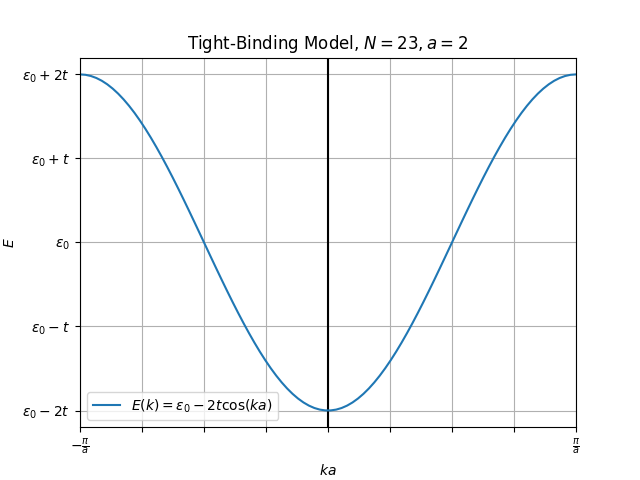
And as we can see, plotted figure perfectly reproduces Figure 11.2 from (Simon, 2013) page 102.

Once we have the theoretical solution plotted, we can solve this system numerically using QuTip and compare them. This consists of defining the Hamiltonian and numerically diagonalizing it. The advantage of using QuTip for it is that it provides us with convenient way of using operators and tensor products which makes it easy to define the Hamiltonian operator.

def _ket(n, N) : return basis(N, n)
def _bra(n, N) : return basis(N, n).dag()

# construct the Hamiltonian
H  = sum([eps*_ket(n, L)*_bra(n, L) for n in range(0, L)])
H -= sum([t*_ket(n, L)*_bra(n + 1, L) for n in range(0, L - 1)])
H -= sum([t*_ket(n, L)*_bra(n - 1, L) for n in range(1, L)])

# solve it numerically
evals, ekets = H.eigenstates()

# satisfy periodic boundary conditions we need E(-k) = E(k)
numerical = np.concatenate((np.flip(evals, 0), evals), axis=0)

let us plot both theoretical and numerical solutions. For theoretical we are going to use same data as in previous plot, while for numerical we will use numerically calculated eigenenergies and we will plot them as red dots.

fig, axs = plt.subplots()
axs.set_xlim(-np.pi/a, np.pi/a)
axs.set_title('Tight-Binding Model, $N='+str(N)+', a='+str(a)+'$')
axs.set_ylabel('$E$')
axs.set_xlabel('$ka$')
axs.axvline(x=0., color='k')
axs.plot(k, numerical, 'ro', label='Eigenvalues of H')
axs.plot(k, exact, label='$E(k) = \epsilon_0 - 2 t \cos(ka)$')
axs.set_yticks([eps-2.*t, eps-t, eps, eps+t, eps+2.*t])
axs.set_yticklabels(['$\epsilon_0-2t$', '$\epsilon_0-t$', '$\epsilon_0$', '$\epsilon_0+t$', '$\epsilon_0+2t$'])
axs.set_xticks(xticks)
axs.set_xticklabels(xlabels)
axs.legend()
axs.grid(True)

Numerical solution for dispersion relation of 1D Tight-Binding Model with lattice spacing of two lattice units. Blue line is the exact solution and red dots are the eigenenergies of the Hamiltonian.

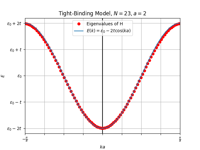
The numerical solution matches theoretical solution closely and reproduces the Figure 11.2 from (Simon, 2013) page 102 perfectly.

The dispersion relation we plotted is essentially a “band”, each of the red dots represents a discrete energy level. With $N$ levels, this energy band can host $2N$ electrons, $N$ for each $k$ value and doubled because of two possible spin orientations. Given a contribution of $2$ electrons from each of the atoms in the 1D lattice that band would be filled completely.

Filling this band completely would cause our 1D chain to be an insulator, filling it partially would make it a conductor.

For the complete source code please consult the gist repository. As usual, if you find anything wrong in the article, any errors etc, feel free to Tweet me and we can fix them!

1. Simon, S. H. (2013). The Oxford solid state basics. Oxford, UK: Oxford Univ. Press.

[Back to Top]