Geometric Phase for a Qubit
Share on:In Physics, the term phase is extremely abused. There could be different phases of matter such as gas phase, liquid phase, solid phase. Changes between them are phase transitions. There also is an idea of a phase space which describes a state of a dynamical system (coordinates are positions and momentum of bodies). The meaning of this term is not very consistent as more generally, a phase represents a state of some periodic function, in Physics that would be a phase of a wave for instance. This leads us to the Mathematical meaning of this concept of a phase which is a complex number of norm taking a form . In the set of phase turns out to be a constant, thus when a physicist tries to sound fancy (phancy!) would say “up to a phase” and what he means is “up to a constant” in .
The geometric phase is (yet another) concept of a phase which results from adiabatic changes in the system which return the system into its initial state and pull out this global phase factor known as geometric phase, Pancharatnam–Berry phase, Pancharatnam phase, or Berry phase. The reason why it has so many names is it was independently discovered by Kato (Kato, 1950) (yet I never heard anyone calling it Kato phase), Pancharatnam (Pancharatnam, 1956), Longuet-Higgins (“Studies of the Jahn-Teller effect .II. The dynamical problem,” 1958) and (the obvious favorite) Sir Michael Berry (“Quantal phase factors accompanying adiabatic changes,” 1984).
In this short tutorial we are going to derive the Berry phase of a qubit after adiabatically traversing a cyclic path on the surface of the Bloch sphere. We are going to derive the expected Berry phase, numerically simulate it and compare the two. This is going to be an adiabatic evolution in a same sense as we did it in Quantum Adiabatic Optimization tutorial.
Let us begin by theoretically deriving the value of such phase. First let us consider a quantum state of a qubit in the Bloch sphere coordinates

assuming the angle is fixed such state would take then the following form
It is straightforward to define this state using QuTip (without -angle dependence)
psi0 = np.cos(theta/2.)*basis(2, 0)+np.sin(theta/2.)*basis(2, 1)
Let that be our initial state for the adiabatic time evolution. We already know implementing the adiabatic evolution requires us to provide the Hamiltonian operator at an arbitrary step of the time evolution in order to let the ground state follow it. The Bloch sphere Hamiltonian for the qubit described in the -basis would take the form
which again is not difficult to implement in QuTip, for instance for varying we can implement the time evolution like this
def sweepPhaseDown(psi0, theta_min, theta_max, phi, tau):
    def angle(t):
        return (1-(t/tau))*theta_max + (t/tau)*theta_min
    res = 300
    times = np.linspace(0., tau, res)
    opts = Options(store_final_state=True)
    H = [
        [sigmax(), (lambda t, args: np.cos(-phi)*np.sin(angle(t)))],
        [sigmay(), (lambda t, args: np.sin(-phi)*np.sin(angle(t)))],
        [sigmaz(), (lambda t, args: np.cos(angle(t)))]]
    return mesolve(H, psi0, times, options=opts)
you may prefer to use lambda functions if your linter allows it! Note that we keep angle in the Hamiltonian which could be simplified using even/odd trigonometric identities, yet I think it is better to keep it this way to indicate the direction of -angle on the Bloch sphere.
So we have the initial state and the Hamiltonian. We know how to evolve it. Now we need something to compare it to, so let us derive the Berry phase. This is done by taking the derivative of state with respect to the angles and
The Berry phase factor
and after the adiabatic time evolution is over the final state will take the form
where is the Berry phase factor and is the dynamic phase factor resulting from the adiabatic time-evolution. We will permit ourselves to ignore by keeping the overall time-evolution length an even multiple of as defined here.
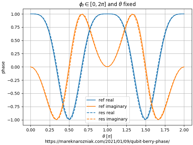
Now let us consider few cases to be numerically tested. For the first plot, we are going to perform a series of numerical time-evolutions initiated in a state . Each of those time evolutions is going to have different initial value of the angle . All of those time-evolutions will perform a full revolution around the Bloch sphere by adiabatically varying the angle from to . The plot below shows the numerically measured value of gemetric phase (dashed line) as well as theoretically predicted value (solid line). The imaginary part is represented by orange and real part by blue.
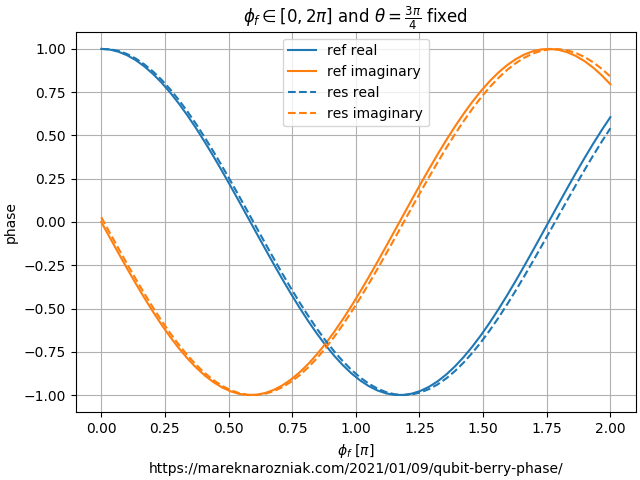
The test consists of another series of numerical time-evolutions initiated in . This time the protocol is slightly different. The angle is increased until it reaches . Then we vary the angle from to and it is the -angle that distinguishes the numerical runs. Each of the runs is finalized by decreasing back to which returns the state back to the North Pole of the Bloch sphere.
The final test consists of three steps just as the previous one, only this time the is fixes and we vary the for each of the adiabatic runs.
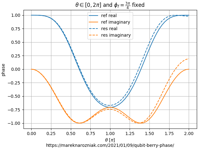
It is visible that that the dash line does not follow solid line closely for the imaginary part for the time-evolution that takes -angle all the way down to the South Pole of the Bloch sphere. I am not sure how to formally prove it, yet my intuition suggests that is the most error-sensitive case as variation of angle while on the South Pole is not reflected by any change of position on the sphere. Moreover, keep in mind state is valid as long as its norm is thus it is the squared value of each of those components that has to add up to . They do seem off by a lot, yet when we square them one gets very close to and another very close to , together they approximate to .
That would be it. I hope you feel more comfortable with this phancy jargon of “phase”. As usual the code is available in this public gist repository and if you have suggestions how to include the dynamical phase in this simulation please feel free to Tweet me and contribute!
- Kato, T. (1950). On the Adiabatic Theorem of Quantum Mechanics. Journal of the Physical Society of Japan, 5(6), 435–439. 10.1143/jpsj.5.435
- Pancharatnam, S. (1956). Generalized theory of interference, and its applications. Proceedings of the Indian Academy of Sciences - Section A, 44(5), 247–262. 10.1007/bf03046050
- Studies of the Jahn-Teller effect .II. The dynamical problem. (1958).Proceedings of the Royal Society of London. Series A. Mathematical and Physical Sciences, 244(1236), 1–16. 10.1098/rspa.1958.0022
- Quantal phase factors accompanying adiabatic changes. (1984).Proceedings of the Royal Society of London. A. Mathematical and Physical Sciences, 392(1802), 45–57. 10.1098/rspa.1984.0023