Constraint Programming

Computer programming is more than having a machine blindly following bunch of rules under the form of computer program. There are many paradigms of programming and constraint logic programming (Jaffar & Lassez, 1987) is a form of nondeterministic programming (Floyd, 1967). Under constraint program, your “program” is a model involving constraints, which is to be processed by a solver searching for solution or a set of solutions to the model.

The constraint satisfaction problem involves a set of variables $\Chi$ , their respective domains $D$ and a set of constraints $C$ that have to be satisfied, putting it all together gives the following structure.

(\Chi, D, C) \tag{CSP}

[diophantine equation over finite domains]

As an example problem, let us define the CSP for solving a particular example of a diophantine equation $x^3+y^2-z^2=0$ over finite domain $[1 \dots 10]$ for each of the variables $x$ , $y$ and $z$ .

\begin{aligned} P &= (\Chi, D, C), \\ \Chi &= \{x, y, z\},\\ D &= \{x \in [1 \dots 10], y \in [1 \dots 10], z \in [1 \dots 10]\},\\ C &= \{x^3+y^2-z^2=0\} \end{aligned}

Easiest way to get started, at least for me, would be to use a simple constraint programming library for Python python-constraint. Let us start by creating empty model, define variables and their finite domains.

from constraint import Problem
problem = Problem()
problem.addVariable('x', range(1, 10))
problem.addVariable('y', range(1, 10))
problem.addVariable('z', range(1, 10))

Define custom constraint that checks if the diophantine equation is satisfied.

def constraintCheck(x, y, z):
    if x**3 + y**2 - z**2 == 0:
        return True
    return False
problem.addConstraint(constraintCheck, ['x', 'y', 'z'])

Process the model and get all the solutions and print them out.

solutions = problem.getSolutions()
for solution in solutions:
    print(solution)
    x = solution['x']
    y = solution['y']
    z = solution['z']
    # you can do something with the values of x, y, z here

This provides us with the following output.

$x$	$y$	$z$
$3$	$3$	$6$
$2$	$1$	$3$

If we plug in those values to $x^3+y^2-z^2=0$ it indeed check out. It is a small but good example showing how powerful constraint programming is for solving the combinatorial problem.

What about optimization problems? What differs constraint satisfaction problem from constraint optimization problem would be the objective function and a criterion. The objective function is a mathematical function accepting assignment of values to variables $\Chi$ withing their respective domains $D$ and returns a number. The criterion is either minimization either maximization, since those are equivalent up to a sign let us just assume from now on we we have minimization by default. If we incorporate those concepts the constraint satisfaction problem will become the constraint optimization problem and what differs them is there is some sort of measure of quality of solution and not all solutions are equivalent, some are preferred over others.

(\Chi, D, C, \text{min} f(\Chi)) \tag{COP}

We have a nice example of problem we could use to define and solve an example constraint optimization problem, we have our Pokémon Centers and Pokémon Gyms problem from Vertex Covers and Independent Sets in game level design and we also have a quantum adiabatic solution to compare from Quantum Adiabatic Optimization. If you haven’t read those tutorials I highly recommend you check them now to know what the problem is about, and if you are already familiar with it, let us proceed with a model.

\begin{aligned} P &= (\Chi, D, C, \text{min} f(\Chi)), \\ \Chi &= \{x_\text{Pallet Town}, x_\text{Viridian City}, \dots x_\text{Cinnabar Island}\},\\ D &= \{x \in \{\text{center}, \text{gym}\} \vert x \in \Chi\},\\ C &= \{\vert\{x_a, x_b\} \cap \{\text{gym}\}\vert \leq 1\vert (x_a, x_b) \in E(G)\},\\ f(\Chi) &= \sum_{x_a \in \Chi} \vert\{x_a\} \cap \{\text{center}\}\vert \end{aligned}

Variables $\Chi$ are towns from Kanto region map from original Pokémon games, their domains $D$ consist of two values - they can be either Pokémon Centers either Pokémon Gyms, finally the constraints enforce the condition of the independent set and we use the the objective function to minimize the overal number of Pokémon centers, effectively solving the minimum vertex cover problem.

As with the previous example, we start by defining empty model.

G = (V, E)
V = list(V)
E = list(E)
problem = Problem()

To define the variables and their domains we follow our definition - every town in Kanto can have either a Pokémon Centers either Pokémon Gyms.

for town in V:
    varname = town.lower().replace(' ', '_')
    problem.addVariable(varname, ['center', 'gym'])

Only one specific constraint is required for each edge of the graph (or each route), it is the independent set constraint - there can be no two Pokémon Gyms next to each other.

for pair in list(E):
    dest_i, dest_j = tuple(pair)
    dest_i = dest_i.lower().replace(' ', '_')
    dest_j = dest_j.lower().replace(' ', '_')
    problem.addConstraint(lambda x, y: True if not x == y == 'gym' else False, [dest_i, dest_j])

We process the model and get the all the CSP solutions

solutions = problem.getSolutions()

Now the tricky part, the python-constraint library does not support constraint optimization problems, so we will have to do a little hack to get the COP solutions - we can filter out the solutions that satisfy the criteria. To make things a bit more fun, we will implement both objective function, the minimum vertex cover and maximum independent set criteria just to check if they match (they must).

best_mis = []
best_mis_size = 0
best_mvc = []
best_mvc_size = len(V) + 1
# get COP solution
for solution in solutions:
    values = list(solution.values())
    nb_gyms = values.count('gym')
    nb_centers = values.count('center')
    # MVC criterion
    if nb_centers < best_mvc_size:
        best_mvc = [solution]
        best_mvc_size = nb_centers
    elif nb_gyms == best_mvc_size:
        best_mvc.append(solution)
    # MIS criterion
    if nb_gyms > best_mis_size:
        best_mis = [solution]
        best_mis_size = nb_gyms
    elif nb_centers == best_mis_size:
        best_mis.append(solution)

Let us this Python trick to check if lists of dictionaries are deeply equal.

assert [i for i in best_mis if i not in best_mvc] == []

If they don’t match that would crash… And it didn’t (you will have to trust me or run by yourself).

Let us continue the tradition and visualize the solutions in retrograming style!

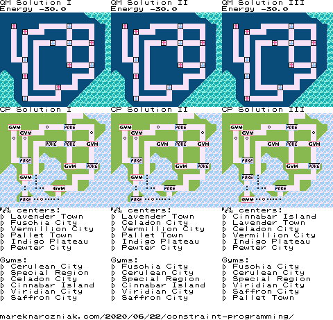
Comparing the quantum solutions to the set theoretical brute force solutions

Totally matches the quantum solution from Quantum Adiabatic Optimization… And from now on let us use COP solution as the reference, it is much smarter way to get solutions than brute force we used in Vertex Covers and Independent Sets in game level design. Even if we hacked around to get the COP criterion processed, which is not very memory efficient, it still should be better. For larger models I highly recommend to use library that already incorporates COP criteria in their search algorithm.

I think that would be it, I decided to keep it brief this time. As usual, if you find errors or typos, or just want to discuss, feel free to tweet me!

For the complete source code please consult the gist repository

Jaffar, J., & Lassez, J.-L. (1987). Constraint Logic Programming. In Proceedings of the 14th ACM SIGACT-SIGPLAN Symposium on Principles of Programming Languages, POPL ’87 (pp. 111–119). New York, NY, USA: Association for Computing Machinery. 10.1145/41625.41635
Floyd, R. W. (1967). Nondeterministic Algorithms. J. ACM, 14(4), 636–644. 10.1145/321420.321422

[Back to Top]