Simulating Superdense Coding with Depolarizing Noise Model

What if I told you that you can transfer two classical bits of information by sending a single quantum bit of information? This is the quantum information theory equivalent of killing two birds with a single stone, known as superdense coding (Bennett & Wiesner, 1992). If you share entangled state with someone you can transfer two classical bits of information by sending a single qubit. This is closely related to quantum teleportation (Bennett et al., 1993) which we already covered earlier.

Recently I’m into combining quantum simulation stuff with retro-game themes, for example when we designed and solved the Vertex Cover problem using brute-force enumeration and also using Quantum Adiabatic Optimization. This tutorial will be no different - we will simulate a quantum information channel based on superdense coding, we will create entanglement and send two bits of information until a GameBoy Classic sprite of Super Mario from Super Mario Land 2 game is completely transferred. We will repeat the process for different depolarizing error probability magnitudes and observe how does it affect our Mario.

The protocol for superdense coding is summarized on following quantum circuit, the middle part ( $X$ and $Z$ gates) are optional and applying them depends on which pair of classical bits we want to encode in single qubit. System involves two qubits, protocol works as follows: the recipient and sender have one qubit each, which are entangled, sender encodes the pair of classical bits in own qubit then sends this single qubit to the recipient who then performs the measurement on the received qubit and own entangled qubit and receives the two classical bits of information.

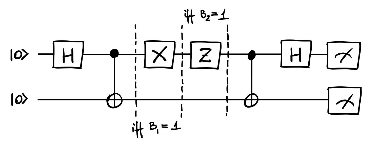
Let us begin by deriving the state after part of the circuit that creates the entanglement, by $H_i$ we denote Hadamard gate applied to $i$ ‘th qubit and by $C^X_{i,j}$ we mean a $\text{CNOT}$ controlled by $i$ ‘th qubit with $j$ ‘th qubit as the target.

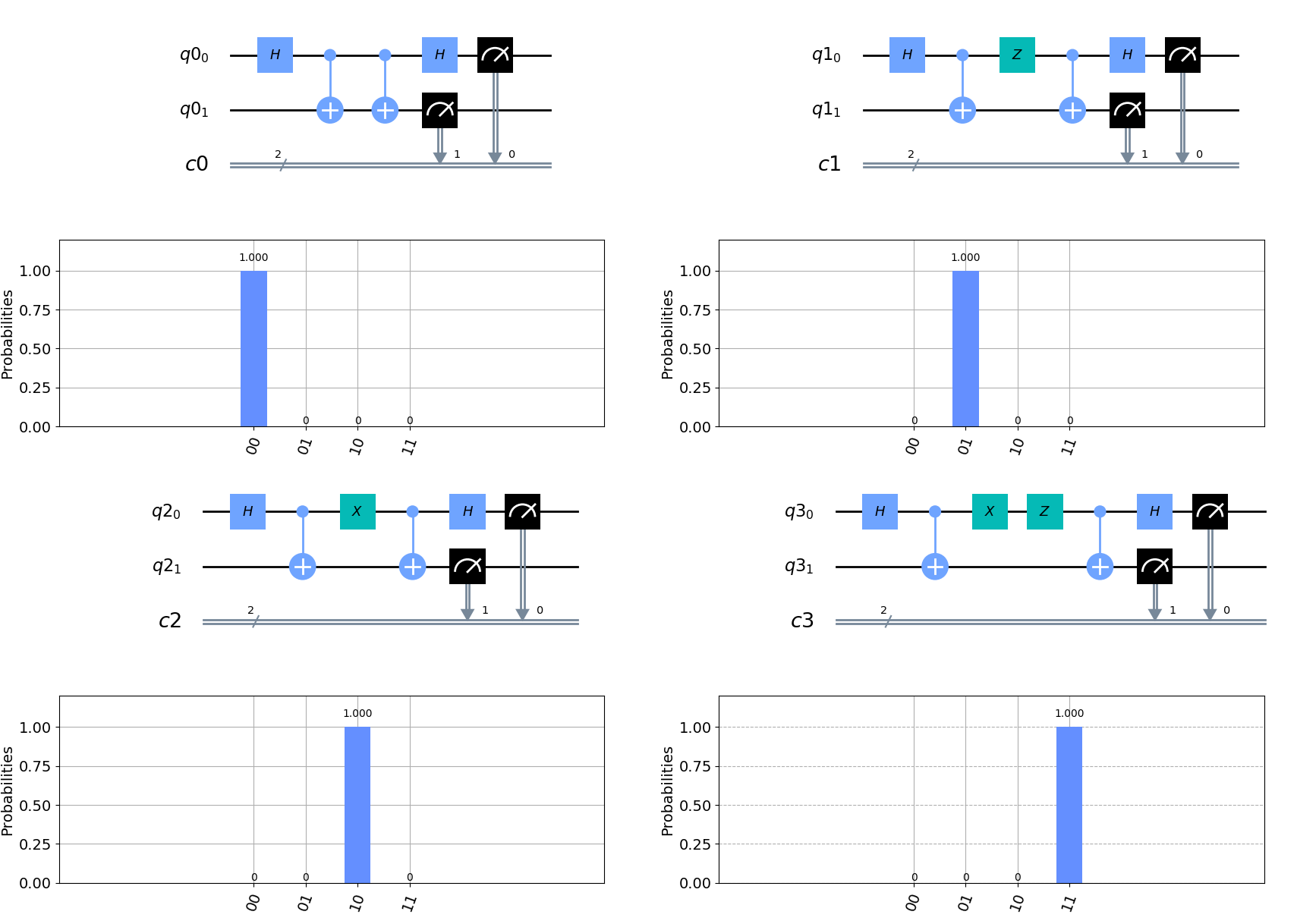
\begin{aligned} C^X_{1,2} H_1 \left| 00 \right> &= C^X_{1,2} \left| +0 \right> \\ &= C^X_{1,2} \frac{1}{\sqrt{2}}(\left| 0 \right> + \left| 1 \right>) \otimes \left| 0 \right> \\ &= C^X_{1,2} \frac{1}{\sqrt{2}}(\left| 00 \right> + \left| 10 \right>)\\ &= \frac{1}{\sqrt{2}}(\left| 00 \right> + \left| 11 \right>)\\ \end{aligned}

Now we consider first case, which is sending classical information of form $00$ , this means we do not apply any gates in the middle of the circuit and we may decode the state directly.

\begin{aligned} H_1 C^X_{1,2}\frac{1}{\sqrt{2}}(\left| 00 \right> + \left| 11 \right>) &= H_1 \frac{1}{\sqrt{2}} (\left|00\right> + \left|10\right>) \\ &= H_1 \frac{1}{\sqrt{2}} (\left|0\right> + \left|1\right>) \otimes \left|0\right> \\ &= H_1 \left|+0\right> \\ &= \left|00\right> \end{aligned}

After reception of the state it is guaranteed to measure $00$ ! Now lets us try sending $10$ , this requires to apply $Z_1$ gate.

\begin{aligned} H_1 C^X_{1,2} Z_1\frac{1}{\sqrt{2}}(\left| 00 \right> + \left| 11 \right>) &= H_1 C^X_{1,2} \frac{1}{\sqrt{2}} (\left|00\right> - \left|11\right>) \\ &= H_1 \frac{1}{\sqrt{2}} (\left|00\right> - \left|10\right>) \\ &= H_1 \frac{1}{\sqrt{2}} (\left|0\right> - \left|1\right>) \otimes \left|0\right> \\ &= H_1 \left|-0\right> \\ &= \left|10\right> \end{aligned}

After reception the $10$ is measured as intended, now sending $01$ , according to the protocol we apply the $X_1$ gate.

\begin{aligned} H_1 C^X_{1,2} X_1\frac{1}{\sqrt{2}}(\left| 00 \right> + \left| 11 \right>) &= H_1 C^X_{1,2} \frac{1}{\sqrt{2}} (\left|10\right> + \left|01\right>) \\ &= H_1 \frac{1}{\sqrt{2}} (\left|11\right> + \left|01\right>) \\ &= H_1 \frac{1}{\sqrt{2}} (\left|1\right> + \left|0\right>) \otimes \left|1\right> \\ &= H_1 \left|+1\right> \\ &= \left|01\right> \end{aligned}

The final case to cover is sending the $11$ classical state, which consists of applying both $X_1$ and $Z_1$ gates.

\begin{aligned} H_1 C^X_{1,2} Z_1 X_1\frac{1}{\sqrt{2}}(\left| 00 \right> + \left| 11 \right>) &= H_1 C^X_{1,2} Z_1\frac{1}{\sqrt{2}} (\left|10\right> + \left|01\right>) \\ &= H_1 C^X_{1,2} \frac{1}{\sqrt{2}} (\left|01\right> - \left|10\right>) \\ &= H_1 \frac{1}{\sqrt{2}} (\left|01\right> - \left|11\right>) \\ &= H_1 \frac{1}{\sqrt{2}} (\left|0\right> - \left|1\right>) \otimes \left|1\right>\\ &= H_1 \left|-1\right>\\ &= \left|11\right>\\ \end{aligned}

To code it upt, lets start by preparing a Python function that makes $N$ qubits and $N$ classical bits empty circuit.

def makeCircuit(N):
    q = QuantumRegister(2)
    c = ClassicalRegister(2)
    qc = QuantumCircuit(q, c)
    return q, c, qc

The superdense coding circuit can be generated automatically based on the two bits of information that are about to be sent.

def superDenseCoding(b1, b2, backend, shots=1024, basis_gates=None, noise_model=None, draw_diagram=False):
    q, c, qc = makeCircuit(2)
    # prepare share entangled state
    qc.h(q[0])
    qc.cx(q[0], q[1])
    # superdense coding operation depend on sended binary bits
    # this part of the circuit is classically controlled
    if b1:
        qc.x(q[0])
    if b2:
        qc.z(q[0])
    # suppose q0 register is sent to receiver
    # decode the transfered information by the receiver
    qc.cx(q[0], q[1])
    qc.h(q[0])
    # measurement
    qc.measure(q, c)
    # build diagram for visualisation
    diagram = None
    if draw_diagram:
        diagram = qc.draw(output="mpl")
    # perform simulation and extract counts
    job = qiskit.execute(
        qc, backend,
        shots=shots,
        basis_gates=basis_gates,
        noise_model=noise_model)
    result = job.result()
    counts = result.get_counts()
    comb = ["".join(seq) for seq in itertools.product('01', repeat=2)]
    for key in comb:
        if key not in counts.keys():
            counts[key] = 0
    # return everything
    return qc, diagram, counts

The output of this function is the simulated quantum circuit, its diagram (if requested by setting draw_diagram=True) and number of measurements for each outcome as a Python’s dictionary object.

When we work with QuTip simulation is slightly different as QuTip by default is simulating circuits in a state vector way, meaning the output is a quantum state and measurements are done by calculating overlaps with different state (or expectation values of an operator object). It is possible to perform this kind of simulation using Qiskit as well, yet by default Qiskit is simulating quantum circuit runs and returns random outcomes, making it closer to an actual experimental approach. This is where the shots parameter becomes relevant, the more shots the greater the resolution of recreating the quantum state outcome probability distribution, which at the limit of shots reaching infinity would become exact. Just as with coin flips, the only way to guarantee having half of flips heads and another half tales is performing an infinite number of throws.

So superdense coding allows you to send two classical bits of information using single quantum bit of information. Now it just so happens that GameBoy Classic screen palette consists of just four colours - so a one pixel is encoded with two bits! Its resolution is $160 \times 144$ pixels, it means that if the GameBoy Classic screen could print from a quantum memory register, hypothetically speaking, it would need $160 \times 144 = 23040$ qubits while for regular bits of information $2 \times 160 \times 144 = 46080$ would be required. The catch here is everything is under assumption we have $23040$ entangled states shared in common prepared upfront (yeah it kind of defies the purpose, but still quite cool to be able to do it!).

Let us simulate a quantum communication channel based on superdense coding we implemented right above and use it to simulate a hypothetical protocol of sending quantum bits of information about sprite to be displayed on a GameBoy Classic screen. For this we can use our superDenseCoding function, because we simulate communication we set shots=1, meaning circuit is run only once or every pixel is sent only once. Every time the generated circuit is run the quantum communication channel is run and sends a pair of classical bits indicated by values of b1 and b2.

def simulateCommunicationChannel(b1, b2, backend, basis_gates=None, noise_model=None):
    _, _, counts = superDenseCoding(b1, b2, backend, shots=1, basis_gates=basis_gates, noise_model=noise_model)
    received_b1 = None
    received_b2 = None
    combinations = list(itertools.product([0, 1], repeat=2))
    for cb1, cb2 in combinations:
        index = str(cb1) + str(cb2)
        if counts[index] == 1:
            received_b1 = cb1
            received_b2 = cb2
    return received_b1, received_b2

As a candidate sprite to be sent via the quantum channel I selected the Mario sprite from Super Mario Land 2 game.

There is really no point in making this article too long and filled with every single line of code, if you are interested in how to prepare this sprite to be sent via the simulated quantum channel then here is how you read the sprite into an array and extract colour palette, here is how you iterate through the sprite and simulate sending pixel by pixel using the superdense coding scheme and finally how you write it back to a new file. It is also pretty important to note that the simplest way is to work with raw bmp bitmap sprites as png, jpeg and other compressed formats contain many parameters you might miss ending up the recreated image look differently even if all the pixels were transferred correctly. To convert a png file into bmp bitmap with $2$ bits per pixel as GameBoy Classic likes it you can use imagemagick library with following command.

convert mario_sprite.png -depth 2 mario_sprite.bmp

Just sending the Mario via the quantum communication channel is not really that exciting, the output is an identical Mario sprite, even if it is using one quantum bit instead of two classical bits, you have to be really nuts about numerical quantum mechanics to feel excited about it, so how about we introduce some quantum errors in the channel and let them perturb our Mario a bit?

Lets introduce the depolarizing error (Wikipedia contributors, 2017) in our quantum communication channel simulation. I use a straightforward example from Qiskit documentation.

from qiskit import Aer
import qiskit.providers.aer.noise as noise

# Error probability
error_prob = 0.1

# Depolarizing quantum errors, single qubit gates
error_1 = noise.depolarizing_error(error_prob, 1)

# two qubit gates
error_2 = noise.depolarizing_error(error_prob, 2)

# initiate a noise model object
noise_model = noise.NoiseModel()

# Add errors to noise model
noise_model.add_all_qubit_quantum_error(error_1, ['u1', 'u2', 'u3'])
noise_model.add_all_qubit_quantum_error(error_2, ['cx'])

# Get basis gates from noise model
basis_gates = noise_model.basis_gates

# Qiskit backend that simulates the circuit
backend = Aer.get_backend('qasm_simulator')

# example how to run the quantum communication channel with the noise model
cb1, cb2 = simulateCommunicationChannel(0, 0, backend, basis_gates, noise_model=noise_model)

Let us push the Mario through the quantum channel and repeat it for different values of depolarizing error probability.

Mario sprite after applying depolarization noise model

The above figure varies the magnitude of depolarization probability from zero to one half. As we can see, when error probability approaches one half there is nearly nothing left of our Mario, it practically turns into noise.

Just few last words before we finish this tutorial, since it is a Qiskit tutorial it is an excellent opportunity to write what I think about their library design.

Terra? Aer? Aqua? Ignis? I did not know Captain Planet works for IBM, what is even more surprising, he is in charge of designing the quantum simulation Python library. Seriously, Qiskit is a really great tool, there are things I like a lot about it, but just this one thing makes me hate it. I find this feng shui design counter-intuitive, annoying and not helpful at all. I do not know if anyone from IBM is reading it, if yes then - change it. Have mercy. I beg you. What if mechanical tools were just named Terra, Aer, Aqua and Ignis? Imagine someone shouting in the warehouse “Hey Mike, bring me the Aer tool” and Mike has to remember that hammer is Aer and Ignis is the drill…

Enough bitching about stuff. I did say there are great things about Qiskit and I meant it, Noise Models is one of the great things, but this naming convention is just so lame I could not stop myself from mentioning it.

That would be it when it comes to this tutorial, as usual if you find some errors, mistakes, typos, do not hesitate to tweet me and let me know!

If you just want some clean superdense coding source for copy-paste and you don’t mind working with Jupyter Notebooks feel free to check up my old homework solution or simply check the gist repository with full source-code from this article.

Bennett, C. H., & Wiesner, S. J. (1992). Communication via one- and two-particle operators on Einstein-Podolsky-Rosen states. Phys. Rev. Lett., 69(20), 2881–2884. 10.1103/PhysRevLett.69.2881
Bennett, C. H., Brassard, G., Crépeau, C., Jozsa, R., Peres, A., & Wootters, W. K. (1993). Teleporting an unknown quantum state via dual classical and Einstein-Podolsky-Rosen channels. Phys. Rev. Lett., 70(13), 1895–1899. 10.1103/PhysRevLett.70.1895
Wikipedia contributors. (2017). Quantum depolarizing channel — Wikipedia, The Free Encyclopedia.

[Back to Top]