Elliptic Curve Cryptography and Diffie-Hellman Key Exchange

The elliptic curve is something I used to hear a lot about and I was almost ashamed for knowing practically nothing about it. Now the time has arrived to clear myself of my ignorance and finally learn what is it all about, and as usual, I wish to share this knowledge on my tech-blog. The use of elliptic curves in cryptography has been independently discovered (Koblitz, 1987; Miller, n.d.). So why the curve? Why elliptic? What does it have to do with cryptography? Let us start with some definition. As for cryptography usage, the elliptic curve is defined as

\begin{aligned} y^2 &= x^3 + ax + b. \end{aligned}

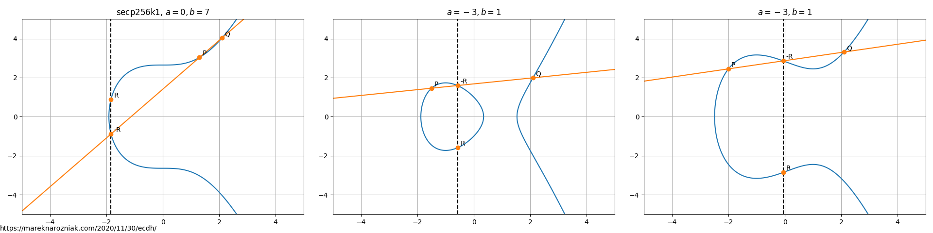
Points belonging to the above equation form a group. The elements of such group are the points of an elliptic curve; the identity element is the point at infinity $0$ ; the inverse of a point is the one symmetric about the -axis; addition is given by the following rule: given three aligned, non-zero points $P = (x_p, y_p)$ and $Q = (x_q, y_q)$ their sum is $R = (x_r, y_r)$ .

\begin{aligned} x_r &= m^2 - x_p - x_q \\ y_r &= y_p + m(x_r - x_p) \end{aligned}

where $m$ is the slope of the line joing the above points

m = \begin{cases} \frac{y_p - y_q}{x_p - x_q}, & \text{if}\ P \neq Q \\ \frac{3 x_p^2 + a}{2 y_p}, & \text{else if}\ P = Q. \end{cases}

Here below please find few examples of curves with points that demonstrate geometric addition on the curve.

We have a well defined addition of two points on the curve, including adding a point to itself. The multiplication by a scalar $n$ follows from the rule of adding a point $n$ times

\begin{aligned} n P &= \sum_{k=1}^n P. \end{aligned}

That was the elliptic curve in real space $\mathbb{R}$ . For cryptographic purposes it is more practical to define the elliptic curve over the finite field $\mathbb{F}_p$ where $p$ is a prime number. Using the modular arithmetic this allows us to perform computation on the curve with finite number of values $p$ . In the finite field representation number of points on the curve is no longer infinite so we do not need to worry about numerical precision. The modular arithmetic provides an equivalence relation, hence we can solve the elliptic curve in the $mod p$ representation and operate on discrete space consisting of a set of $p$ points. The reason why $p$ has to be a prime number is that is a requirement for $\mathbb{F}_p$ to satisfy the field axioms. The figures below compare same curve secp256k1 over real space $\mathbb{R}$ and over finite field $\mathbb{F}_p$ where $p = 17$ .

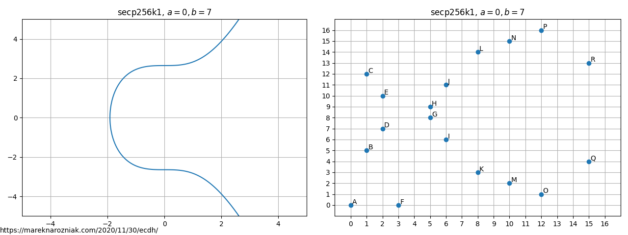
As visible on the figure, the finite field $\mathbb{F}_p$ representation looks nothing like a curve. It does inherit the label “curve” but it does not have to look like a curve. It does solve curve equation over finite field and that is the only reason we call it this way. The point belongs to the curve over finite field if it satisfies the following equation

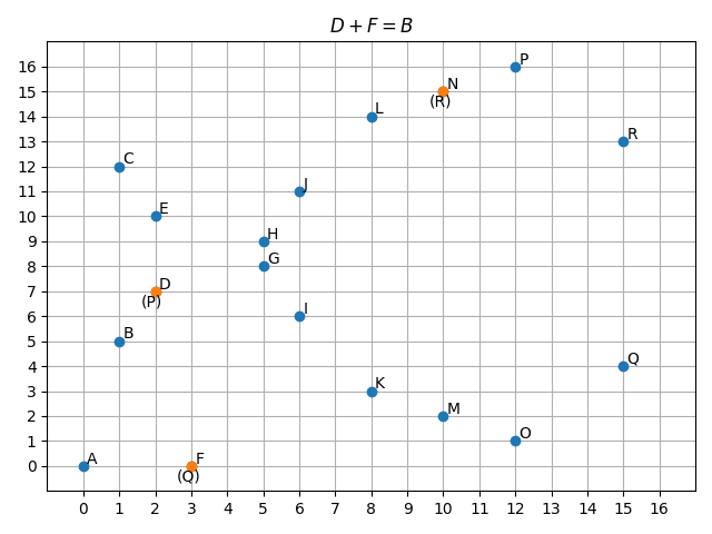
\begin{aligned} (y^2 - x^3 - ax - b) \mod p &= 0 \end{aligned}

The addition and multiplication by a scalar still work in the modular arithmetic. For calculating the inverse we use the modular multiplicative inverse which relies on the Extended Euclidean algorithm. As an example, here below we add points labeled by $D$ and $F$ in order to compute $D + F = B$ .

We can add points that lay on the curve in the $\mathbb{F}_p$ space and resulting point will always remain in this space. It is the same in with multiplying them by a scalar $n$ . The addition is implemented in Python as follows

def eccFiniteAddition(Px, Py, Qx, Qy, a, b, p):
    if None in [Px, Py]:
        return Qx, Qy
    if None in [Qx, Qy]:
        return Px, Py
    if Px == Qx and Py != Qy:
        # point1 + (-point1) = 0
        return None, None
    if Px == Qx:
        m = (3*Px**2 + a)*inverse(2*Py, p)
    else:
        m = (Py - Qy)*inverse(Px - Qx, p)
    Rx = np.mod(m**2 - Px - Qx, p)
    Ry = np.mod(-(Py + m*(Rx - Px)), p)
    return Rx, Ry

and multiplication follows from it

def eccScalarMult(k, Px, Py, a, b, p):
    assert onCurve(Px, Py, a, b, p)
    if np.mod(k, p) == 0:
        return None, None
    if k < 0:
        # k * point = -k * (-point)
        Rx, Ry = eccNegation(Px, Py)
        return eccScalarMult(-k, Rx, Ry)
    rx, ry = Px, Py
    for i in range(k):
        rx, ry = eccFiniteAddition(rx, ry, Px, Py, a, b, p)
    return rx, ry

where eccNegation negates the point on the curve and the inverse implements the modular multiplicative inverse algorithm. Those are defined in gist dedicated for this article.

We can also control the size of this discrete space by choosing $p$ prime number of appropriate magnitude. Now what is the motivation of that? What is so great about it? The advantage of that is, we can efficiently calculate sums and products, but we cannot efficiently divide points from this space. If you wonder why, I challenge you to pick two points $P$ and $Q$ on the elliptic curve in finite field graph and try to find a constant number of additions $k$ such that $k P = Q$ . You will end up blindly trying all possible values of $k$ until you find one that works, which is not a deterministic approach. This indicates group formed by the elliptic curve implements a trapdoor function which works efficiently one way around but not the other way around. A bit similar as we did in our satisfiability article but much more efficietly! Let us illustrate a practical use-case of that by introducing the Diffie-Hellman Key Exchange protocol (Merkle, 1978; Diffie & Hellman, 1976).

Let us imagine Alice and Bob want to establish a secure communication via an unsafe channel. A third participant - Charlie - is constantly checking all their messages (yes, Charlie the unicorn). Both Alice and Bob agree on the key size which in this case is the prime number $p$ . The larger, the better security as it increases the size of the $\mathbb{F}_p$ space. They also agree on a generator $G$ which is a point in the $\mathbb{F}_p$ space. They also both chose their private key, which is simply a scalar number, for Alice let us call it $k_A$ and for Bob $k_B$ . In principle, because addition is associative we can expect the following to hold

\begin{aligned} k_A (k_B G) &= (k_A G) k_B \end{aligned}

and this is what makes the Diffie-Hellman key exchange work! So Alice and Bob both calculate their public keys $p_A$ and $p_B$ using elliptic curve arithmetics

\begin{aligned} p_A &= k_A G \\ p_B &= k_B G \end{aligned}

and they exchange their public keys via the insecure channel. Lets say that the generator point $G = Q$ in our $\mathbb{F}_p$ with $p = 17$ . Computation process is demonstrated by a series of transitions $k_A$ or $k_B$ in the $\mathbb{F}_p$ space originating at the generator point $G = Q$ (in green) and leading to the public key point (in orange).

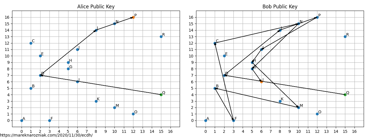
So in this space Alice public key is $p_A = H$ and Bobs $p_B = O$ . Charlie listened to everything and he knows $G$ , $p$ , $p_A$ , $p_B$ but he does not know $k_A$ nor $k_B$ . Now both Alice and Bob multiply each others public keys by own private key which is again visualized using series of transitions.

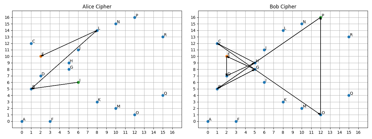
As visible on the figure, both Alice and Bob found exactly the same point $C$ through completely different paths! Charlie does not know the point $C$ . In Elliptic Curve Cryptography it is not possible to use public key directly for encryption, however both Alice and Bob can use the shared secret for bulk encryption algorithms such as AES.

Now Charlie could try to brute-force the private key from the public key

def bruteForceKey(Px, Py, pub_x, pub_y, a, b, p):
    for k in range(p):
        _, _, public_x, public_y = eccScalarMult(k, Px, Py, a, b, p)
        if public_x == pub_x and public_y == pub_y:
            return k

which applied to our above example gives the following (correct) result

Bob private key:  13
Alice private key:  4

In practice, however, the key size $p$ is supposed to be a huge number eliminating the possibility of brute-forcing the key. If you find a deterministic algorithm that finds the multiplication scalar based on two points on the elliptic curve you would solve the discrete logarithm problem.

To wrap it up I would like to share few excellent articles that I used while learning about the elliptic curve and preparing the coding examples. I recommend the Practical Cryptography for Developers book as well as the gentle introduction, finite fields and the excellent interactive tool by Andrea Corbellini. I also recommend these animated examples by @xargsnotbombs Michael Driscoll. My examples and code are heavily based on those materials and I highly recommend you check read them for more information. The repository with source-code that renders all the plots is available in this public gist repository. As usual, if you find typos, errors, something is not clear, something is wrong, do not hesitate to let me know and feel free to tweet me!

Koblitz, N. (1987). Elliptic curve cryptosystems. Mathematics of Computation, 48(177), 203–203. 10.1090/s0025-5718-1987-0866109-5
Miller, V. S. Use of Elliptic Curves in Cryptography. In Lecture Notes in Computer Science (pp. 417–426). Springer Berlin Heidelberg. 10.1007/3-540-39799-x_31
Merkle, R. C. (1978). Secure communications over insecure channels. Communications of the ACM, 21(4), 294–299. 10.1145/359460.359473
Diffie, W., & Hellman, M. (1976). New directions in cryptography. IEEE Transactions on Information Theory, 22(6), 644–654. 10.1109/tit.1976.1055638

[Back to Top]