Simulating Quantum Teleportation

Initially introduced in (Bennett et al., 1993), a quantum teleportation describes a protocol allowing to reconstruct an unknown quantum state $\vert \psi >$ at a new location by using classical information channel and a pair of entangled states.

The word teleportation does fit well here as this phenomenon occurs instantaneously and is not affected by distance or separating barriers. The instantaneously teleported state cannot be used to achieve faster than light communication, as in order to be properly reconstructed requires classical information about measurement performed at the sender location, making it sensitive to limitations imposed by the speed of light.

Quantum teleportation requires three qubits, where first one holds the state to be teleported and the remaining ones are initialised to $\left \vert 0 \right>$, and consists of performing the following quantum circuit.

Quantum circuit performing teleportation of an arbitrary state. Creating the entanglement is included.

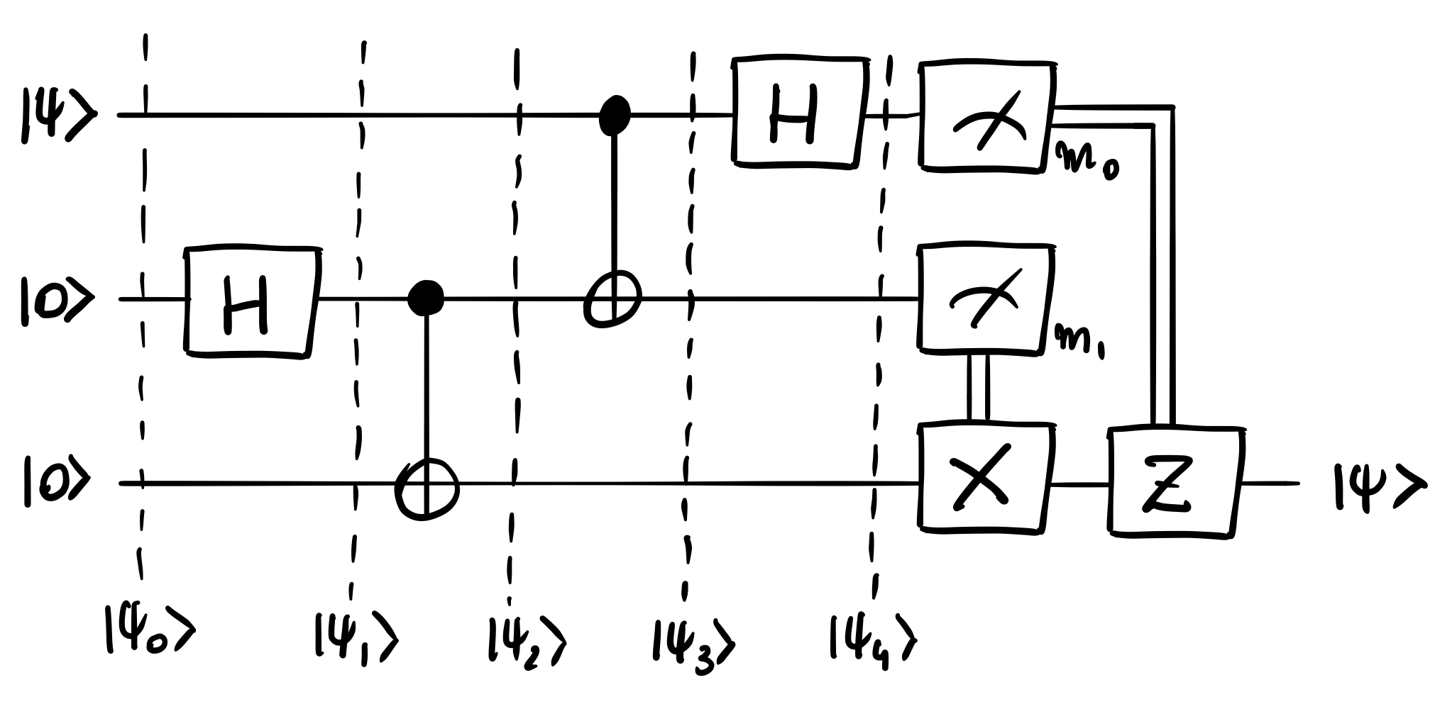
Let us derive the quantum state at each of those steps. We denote a $\text{CNOT}$-gate with control qubit $c$ and target qubit $t$ by $C^c_t$ and a Hadamard gate with target $t$ as $H_t$. We are going to teleport a quantum state of a general form $\alpha \left \vert 0 \right > + \beta \left \vert 1 \right >$.

$\begin{aligned} \left \vert \psi_0 \right > &= (\alpha \left \vert 0 \right > + \beta \left \vert 1 \right >) \otimes \left \vert 00 \right > \\ &= \alpha \left \vert 000 \right > + \beta \left \vert 100 \right > \end{aligned}$

We apply the first Hadamard gate to the middle qubit.

$\begin{aligned} H_2 \left \vert \psi_0 \right > &= \alpha \left \vert 0+0 \right > + \beta \left \vert 1+0 \right > \\ &= \frac{1}{\sqrt{2}} (\alpha \left \vert 000 \right > + \alpha \left \vert 010 \right > + \beta \left \vert 100 \right > + \beta \left \vert 110 \right >) \\ &= \left \vert \psi_1 \right > \end{aligned}$

Step that follows is a $\text{CNOT}$-gate with third qubit as a target and middle superposition qubit as control.

$\begin{aligned} C_2^3 \left \vert \psi_1 \right > &= \frac{1}{\sqrt{2}} (\alpha \left \vert 000 \right > + \alpha \left \vert 011 \right > + \beta \left \vert 100 \right > + \beta \left \vert 111 \right >) \\ &= \left \vert \psi_2 \right > \end{aligned}$

This completes the creation of the entangled state between second and third qubit. Now we can apply the actual teleportation, starting from another $\text{CNOT}$-gate with qubit to be teleported as control and middle qubit as target.

$\begin{aligned} C_1^2 \left \vert \psi_2 \right > &= \frac{1}{\sqrt{2}} (\alpha \left \vert 000 \right > + \alpha \left \vert 011 \right > + \beta \left \vert 110 \right > + \beta \left \vert 101 \right >) \\ &= \left \vert \psi_3 \right > \end{aligned}$

The final Hadamard gate applied to to-be-teleported state completes the teleportation procedure. Let us write it in a nicely factored form.

$\begin{aligned} H_1 \left \vert \psi_2 \right > &= \frac{1}{2} \left \vert 00 \right > (\alpha \left \vert 0 \right > + \beta \left \vert 1 \right >) + \frac{1}{2} \left \vert 01 \right > (\alpha \left \vert 1 \right > + \beta \left \vert 0 \right >) + \frac{1}{2} \left \vert 10 \right > (\alpha \left \vert 0 \right > - \beta \left \vert 1 \right >) + \frac{1}{2} \left \vert 11 \right > (\alpha \left \vert 1 \right > - \beta \left \vert 0 \right >) \\ &= \left \vert \psi_4 \right > \end{aligned}$

In this form it is visible what gates have to applied to the last qubit to make it match the input teleported state $\alpha \left \vert 0 \right > + \beta \left \vert 1 \right >$. The gates to be applied depend on the measurement of the first two qubits as teleported state is still entangled with them. That is the motivation behind the idea of classical correction.

Now lets simulate this protocol. I would like to keep this tutorial as practical as possible, for the complete source code please consult the gist repository, and no more bla bla, lets get this teleportation started by importing required dependencies.

import numpy as np

import itertools

from qutip import basis, tensor, rand_ket, snot, cnot, rx, rz, qeye

We create a random two-level state $\left \vert \psi \right >$ to be teleported.

psi = rand_ket(2)

The initial state for entire teleportation circuit can be defined as $\left \vert \psi_0 \right> = \left \vert \psi \right > \otimes \left \vert 0 \right > \otimes \left \vert 0 \right >$ and QuTip provides us with a convenient way of writing that down as follows

psi0 = tensor([psi, basis(2, 0), basis(2, 0)])

We can realise this circuit as sequence of unitary operations as follows.

psi1 = snot(N=3, target=1)*psi0
psi2 = cnot(N=3, control=1, target=2)*psi1
psi3 = cnot(N=3, control=0, target=1)*psi2
psi4 = snot(N=3, target=0)*psi3

Applying classical correction is not easy if we work with state vectors, we will do it by projecting particular measurement outcomes of the first two qubits, which will result with four possible outcomes, then to each of those outcomes we can apply an appropriate correction.

Lets prepare the four projection operators, one for each of those outcomes. This process can be automated by generating all the possible measurement outcomes of two qubits by using the itertools library.

confs = list(itertools.product([0, 1], repeat=2))

Ps = []
for m0, m1 in confs:
    P = tensor([
        basis(2, m0).proj(),
        basis(2, m1).proj(),
        qeye(2)])
    Ps.append(P)

Finally, we can use those operators to get the projected state and in this way simulating the measurement of the first two qubits.

The way it works is, given state $\left \vert \psi_4 \right>$ we can create a state $\left \vert \psi_{ij} \right>$ which is interpreted as “$\left \vert \psi_{ij} \right>$ is $\left \vert \psi_4 \right>$ after measuring $i$ on first qubit and $j$ on the second qubit”. We can get is as follows

$P_{ij} \left \vert \psi_4 \right> = \left \vert \psi_{ij} \right>$

Lets use qubit to calculate those projected states. Don’t forget to normalize!

psis_proj = []
for P in Ps:
    psi_proj = (P*psi4).unit()
    psis_proj.append(psi_proj)

From the figure we know what classical correction should be applied to each outcome: for $\left\vert00\right>$ measurement we do not apply any correction, for $\left\vert01\right>$ we apply $X$-correction, for $\left\vert10\right>$ we apply the $Z$-correction and finally for $\left\vert11\right>$ we apply both $X,Z$-corrections.

Let’s prepare those operators.

X = rx(np.pi, N=3, target=2)
Z = rz(np.pi, N=3, target=2)

We have states for each of the possible measurement outcomes and adequate operators, we also know which operator to apply in case of which outcome has been measured so all we have to do is apply them. For the notation, lets assume that $\left \vert \psi^c_{ij} \right >$ will be the corrected state $\left \vert \psi_{ij} \right >$.

psis_corr = [
    psis_proj[0],
    X*psis_proj[1],
    Z*psis_proj[2],
    Z*X*psis_proj[3]
]

Now we can check if the state has been properly corrected by calculating the fidelity of each of those outcomes, to do it we will need set of reference states, each of the form

$\left\vert \psi^e_{ij} \right > = \left \vert i \right > \otimes \left \vert j \right > \otimes \left \vert \psi \right >$

This form captures what was we assumed has been measured, as well as what we expect to have in the third qubit - the correctly teleported state. Lets prepare the expected reference states.

psis_ref = []
for m0, m1 in confs:
    psi_ref = tensor([basis(2, m0), basis(2, m1), psi])
    psis_ref.append(psi_ref)

Now we can calculate and display the fidelities, we do so by taking the overlap of what has been measured with what has been expected to be measured and absolute value square it to get the probability of measuring what we want to measure.

$\vert\left< \psi^e_{ij} \vert \psi^c_{ij} \right >\vert^2$

Calculating those fidelities and printing them out along with the associated measurements of first two qubits can be done as follows.

print('{0:2} {1:2} {2:8}'.format('m0', 'm1', 'fidelity'))
for conf, psi_corr, psi_ref in zip(confs, psis_corr, psis_ref):
    fidelity = np.round(np.abs(psi_corr.overlap(psi_ref))**2., 3)
    m0, m1 = conf
    print('{0:2} {1:2} {2:8}'.format(m0, m1, fidelity))

Displays the following output

m0 m1 fidelity
 0  0      1.0
 0  1      1.0
 1  0      1.0
 1  1      1.0

So for each of the outcomes we can see the probability of measuring the teleported state on the third qubit. We also play a bit and see what those probabilities would be if we did not apply the classical correction (an attempt for faster than light communication!).

Easy to check! Just use the non-corrected states!

print('{0:2} {1:2} {2:8}'.format('m0', 'm1', 'fidelity'))
for conf, psi_proj, psi_ref in zip(confs, psis_proj, psis_ref):
    fidelity = np.round(np.abs(psi_proj.overlap(psi_ref))**2., 3)
    m0, m1 = conf
    print('{0:2} {1:2} {2:8}'.format(m0, m1, fidelity))

Displays the following output

m0 m1 fidelity
 0  0      1.0
 0  1    0.166
 1  0    0.349
 1  1    0.485

So, if the measurement outcome on first two qubits is $\left \vert 00 \right >$ then fidelity is good but note that this also happens to be the case that requires no correction!

Bar plot showing how unreliable teleportation is without the classical correction.

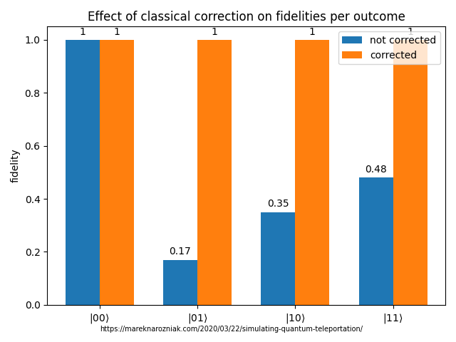
Our faster than light communication is not very reliable, would work only assuming the first two qubits get this particular measurement outcome and in general case would lead the person on the other side of the universe to receive a random noise instead of the message that was intended to be received.

I hope you enjoyed this tutorial and I also hope it will encourage you to give QuTip a shot (if you haven’t yet), its a really great library full of wonderful tools which make work with quantum mechanical simulation a lot more pleasant.

1. Bennett, C. H., Brassard, G., Crépeau, C., Jozsa, R., Peres, A., & Wootters, W. K. (1993). Teleporting an unknown quantum state via dual classical and Einstein-Podolsky-Rosen channels. Phys. Rev. Lett., 70(13), 1895–1899. 10.1103/PhysRevLett.70.1895

[Back to Top]